Note

This page is a reference documentation. It only explains the class signature, and not how to use it. Please refer to the user guide for the big picture.

nilearn.plotting.displays.OrthoSlicer¶

class nilearn.plotting.displays.OrthoSlicer(cut_coords, axes=None, black_bg=False, brain_color=(0.5, 0.5, 0.5), **kwargs)[source]¶

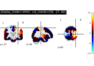
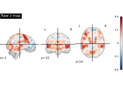
Class to create 3 linked axes for plotting orthogonal cuts of 3D maps.

This visualization mode can be activated from Nilearn plotting functions, like plot_img, by setting display_mode='ortho':

from nilearn.datasets import load_mni152_template
from nilearn.plotting import plot_img

img = load_mni152_template()
# display is an instance of the OrthoSlicer class
display = plot_img(img, display_mode="ortho")

Attributes:

cut_coordslist: The cut coordinates.
axesdict of Axes: The 3 axes used to plot each view.
frame_axesAxes: The axes framing the whole set of views.

See also

nilearn.plotting.displays.MosaicSlicer: Three cuts are performed along multiple rows and columns.
nilearn.plotting.displays.TiledSlicer: Three cuts are performed and arranged in a 2x2 grid.

Notes

The extent of the different axes are adjusted to fit the data best in the viewing area.

__init__(cut_coords, axes=None, black_bg=False, brain_color=(0.5, 0.5, 0.5), **kwargs)[source]¶

classmethod find_cut_coords(img=None, threshold=None, cut_coords=None)[source]¶

Instantiate the slicer and find cut coordinates.

Parameters:

imgNiimg-like object

See Input and output: neuroimaging data representation.

thresholdint or float or None, default=None

Threshold to apply:

If None is given, the maps are not thresholded.

If a number is given, it is used to threshold the maps, values below the threshold (in absolute value) are plotted as transparent.

cut_coords3 tuple of int

The cut position, in world space.

draw_cross(cut_coords=None, **kwargs)[source]¶

Draw a crossbar on the plot to show where the cut is performed.

Parameters:

cut_coords3-tuple of float, optional: The position of the cross to draw. If None is passed, the OrthoSlicer’s cut coordinates are used.
kwargsdict: Extra keyword arguments are passed to function axhline.

add_contours(img, threshold=1e-06, filled=False, **kwargs)[source]¶

Contour a 3D map in all the views.

Parameters:

imgNiimg-like object

See Input and output: neuroimaging data representation. Provides image to plot.

thresholdint or float or None, default=1e-6

Threshold to apply:

If None is given, the maps are not thresholded.

If a number is given, it is used to threshold the maps, values below the threshold (in absolute value) are plotted as transparent.

filledbool, default=False

If filled=True, contours are displayed with color fillings.

kwargsdict

Extra keyword arguments are passed to function contour, or function contourf. Useful, arguments are typical “levels”, which is a list of values to use for plotting a contour or contour fillings (if filled=True), and “colors”, which is one color or a list of colors for these contours.

Notes

If colors are not specified, default coloring choices (from matplotlib) for contours and contour_fillings can be different.

add_edges(img, color='r')[source]¶

Plot the edges of a 3D map in all the views.

Parameters:

imgNiimg-like object: See Input and output: neuroimaging data representation. The 3D map to be plotted. If it is a masked array, only the non-masked part will be plotted.
colormatplotlib color: str or (r, g, b) value, default=’r’: The color used to display the edge map.

add_markers(marker_coords, marker_color='r', marker_size=30, **kwargs)[source]¶

Add markers to the plot.

Parameters:

marker_coordsndarray of shape (n_markers, 3): Coordinates of the markers to plot. For each slice, only markers that are 2 millimeters away from the slice are plotted.
marker_colorpyplot compatible color or list of shape (n_markers,), default=’r’: List of colors for each marker that can be string or matplotlib colors.
marker_sizefloat or list of float of shape (n_markers,), default=30: Size in pixel for each marker.

add_overlay(img, threshold=1e-06, colorbar=False, cbar_tick_format='%.2g', cbar_vmin=None, cbar_vmax=None, **kwargs)[source]¶

Plot a 3D map in all the views.

Parameters:

imgNiimg-like object

See Input and output: neuroimaging data representation. If it is a masked array, only the non-masked part will be plotted.

thresholdint or float or None, default=1e-6

Threshold to apply:

If None is given, the maps are not thresholded.

If a number is given, it is used to threshold the maps: values below the threshold (in absolute value) are plotted as transparent.

cbar_tick_format: str, default=”%.2g” (scientific notation)

Controls how to format the tick labels of the colorbar. Ex: use “%i” to display as integers.

colorbarbool, default=False

If True, display a colorbar on the right of the plots.

kwargsdict

Extra keyword arguments are passed to function imshow.

cbar_vminfloat, optional

Minimal value for the colorbar. If None, the minimal value is computed based on the data.

cbar_vmaxfloat, optional

Maximal value for the colorbar. If None, the maximal value is computed based on the data.

annotate(left_right=True, positions=True, scalebar=False, size=12, scale_size=5.0, scale_units='cm', scale_loc=4, decimals=0, **kwargs)[source]¶

Add annotations to the plot.

Parameters:

left_rightbool, default=True

If True, annotations indicating which side is left and which side is right are drawn.

positionsbool, default=True

If True, annotations indicating the positions of the cuts are drawn.

scalebarbool, default=False

If True, cuts are annotated with a reference scale bar. For finer control of the scale bar, please check out the draw_scale_bar method on the axes in “axes” attribute of this object.

sizeint, default=12

The size of the text used.

scale_sizeint or float, default=5.0

The length of the scalebar, in units of scale_units.

scale_units{‘cm’, ‘mm’}, default=’cm’

The units for the scalebar.

scale_locint, default=4

The positioning for the scalebar. Valid location codes are:

1: “upper right”

2: “upper left”

3: “lower left”

4: “lower right”

5: “right”

6: “center left”

7: “center right”

8: “lower center”

9: “upper center”

10: “center”

decimalsint, default=0

Number of decimal places on slice position annotation. If zero, the slice position is integer without decimal point.

kwargsdict

Extra keyword arguments are passed to matplotlib’s text function.

property black_bg¶: Return black background.

property brain_color¶: Return brain color.

close()[source]¶

Close the figure.

This is necessary to avoid leaking memory.

classmethod init_with_figure(img, threshold=None, cut_coords=None, figure=None, axes=None, black_bg=False, leave_space=False, colorbar=False, brain_color=(0.5, 0.5, 0.5), **kwargs)[source]¶

Initialize the slicer with an image.

Parameters:

imgNiimg-like object: See Input and output: neuroimaging data representation.
cut_coords3 tuple of int: The cut position, in world space.
axesmatplotlib.axes.Axes, optional: The axes that will be subdivided in 3.
black_bgbool, default=False: If True, the background of the figure will be put to black. If you wish to save figures with a black background, you will need to pass facecolor='k', edgecolor='k' to matplotlib.pyplot.savefig.
brain_colortuple, default=(0.5, 0.5, 0.5): The brain color to use as the background color (e.g., for transparent colorbars).

savefig(filename, dpi=None)[source]¶

Save the figure to a file.

Parameters:

filenamestr: The file name to save to. Its extension determines the file type, typically ‘.png’, ‘.svg’ or ‘.pdf’.
dpiNone or scalar, default=None: The resolution in dots per inch.

title(text, x=0.01, y=0.99, size=15, color=None, bgcolor=None, alpha=1, **kwargs)[source]¶

Write a title to the view.

Parameters:

textstr: The text of the title.
xfloat, default=0.01: The horizontal position of the title on the frame in fraction of the frame width.
yfloat, default=0.99: The vertical position of the title on the frame in fraction of the frame height.
sizeint, default=15: The size of the title text.
colormatplotlib color specifier, optional: The color of the font of the title.
bgcolormatplotlib color specifier, optional: The color of the background of the title.
alphafloat, default=1: The alpha value for the background.
kwargs: Extra keyword arguments are passed to matplotlib’s text function.

Examples using `nilearn.plotting.displays.OrthoSlicer`¶

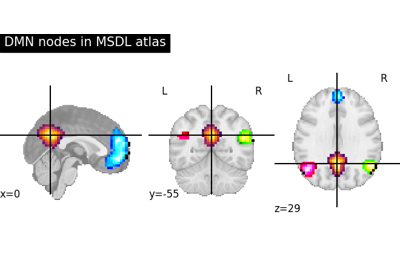
Visualizing a probabilistic atlas: the default mode in the MSDL atlas

More plotting tools from nilearn

Producing single subject maps of seed-to-voxel correlation

Regions extraction using dictionary learning and functional connectomes

Default Mode Network extraction of ADHD dataset

Statistical testing of a second-level analysis

Beta-Series Modeling for Task-Based Functional Connectivity and Decoding

nilearn.plotting.displays.OrthoSlicer¶

Examples using nilearn.plotting.displays.OrthoSlicer¶

Examples using `nilearn.plotting.displays.OrthoSlicer`¶