Plotting tools in nilearn

Nilearn comes with a set of plotting functions for easy visualization of Nifti-like images such as statistical maps mapped onto anatomical images or onto glass brain representation, anatomical images, functional/EPI images, region specific mask images.

See Plotting brain images for more details.

We will first retrieve data from nilearn provided (general-purpose) datasets.

from nilearn import datasets

# haxby dataset to have EPI images and masks
haxby_dataset = datasets.fetch_haxby()

# print basic information on the dataset
print(
    f"First subject anatomical nifti image (3D) is at: {haxby_dataset.anat[0]}"
)
print(
    f"First subject functional nifti image (4D) is at: {haxby_dataset.func[0]}"
)

haxby_anat_filename = haxby_dataset.anat[0]
haxby_mask_filename = haxby_dataset.mask_vt[0]
haxby_func_filename = haxby_dataset.func[0]

# one motor activation map
stat_img = datasets.load_sample_motor_activation_image()

[fetch_haxby] Dataset found in /home/runner/nilearn_data/haxby2001
First subject anatomical nifti image (3D) is at: /home/runner/nilearn_data/haxby2001/subj2/anat.nii.gz
First subject functional nifti image (4D) is at: /home/runner/nilearn_data/haxby2001/subj2/bold.nii.gz

Nilearn plotting functions

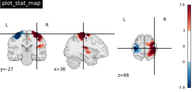
Plotting statistical maps: plot_stat_map

from nilearn import plotting

Visualizing t-map image on EPI template with manual positioning of coordinates using cut_coords given as a list

plotting.plot_stat_map(
    stat_img, threshold=3, title="plot_stat_map", cut_coords=[36, -27, 66]
)

<nilearn.plotting.displays._slicers.OrthoSlicer object at 0x7f0f561913c0>

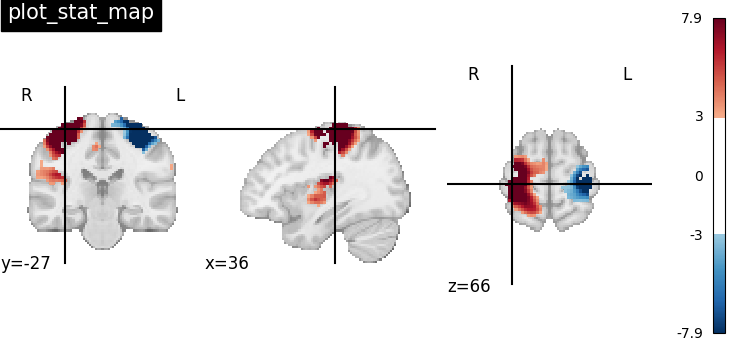
It’s also possible to visualize volumes in a LR-flipped “radiological” view Just set radiological=True

plotting.plot_stat_map(
    stat_img,
    threshold=3,
    title="plot_stat_map",
    cut_coords=[36, -27, 66],
    radiological=True,
)

<nilearn.plotting.displays._slicers.OrthoSlicer object at 0x7f0f55dfb610>

Making interactive visualizations: view_img

An alternative to plot_stat_map is to use view_img that gives more interactive visualizations in a web browser. See Interactive visualization of statistical map slices for more details.

from nilearn.plotting import view_img

view = view_img(stat_img, threshold=3)
# In a notebook, if ``view`` is the output of a cell, it will
# be displayed below the cell
view

/home/runner/work/nilearn/nilearn/.tox/doc/lib/python3.10/site-packages/numpy/_core/fromnumeric.py:868: UserWarning: Warning: 'partition' will ignore the 'mask' of the MaskedArray.
  a.partition(kth, axis=axis, kind=kind, order=order)

uncomment this to open the plot in a web browser: view.open_in_browser()

It’s also possible to visualize volumes in a LR-flipped “radiological” view Just set radiological=True

view_radio = view_img(
    stat_img, threshold=3, title="radiological view", radiological=True
)
view_radio

/home/runner/work/nilearn/nilearn/.tox/doc/lib/python3.10/site-packages/numpy/_core/fromnumeric.py:868: UserWarning: Warning: 'partition' will ignore the 'mask' of the MaskedArray.
  a.partition(kth, axis=axis, kind=kind, order=order)

uncomment this to open the plot in a web browser: view_radio.open_in_browser()

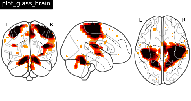
Plotting statistical maps in a glass brain: plot_glass_brain

Now, the t-map image is mapped on glass brain representation where glass brain is always a fixed background template

plotting.plot_glass_brain(stat_img, title="plot_glass_brain", threshold=3)

<nilearn.plotting.displays._projectors.OrthoProjector object at 0x7f0f31b62e90>

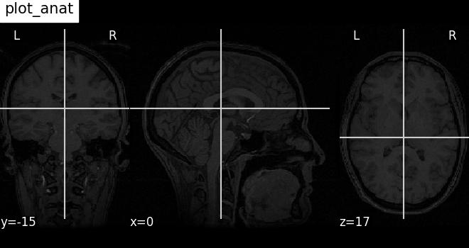
Plotting anatomical images: plot_anat

Visualizing anatomical image of haxby dataset

plotting.plot_anat(haxby_anat_filename, title="plot_anat")

<nilearn.plotting.displays._slicers.OrthoSlicer object at 0x7f0f33b5a620>

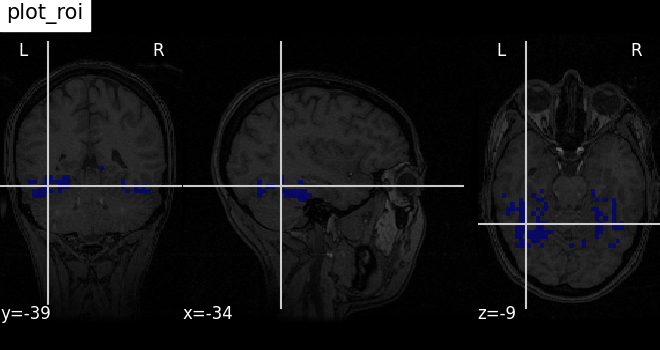
Plotting ROIs (here the mask): plot_roi

Visualizing ventral temporal region image from haxby dataset overlaid on subject specific anatomical image with coordinates positioned automatically on region of interest (roi)

plotting.plot_roi(
    haxby_mask_filename, bg_img=haxby_anat_filename, title="plot_roi"
)

<nilearn.plotting.displays._slicers.OrthoSlicer object at 0x7f0f55df96c0>

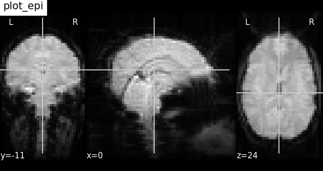
Plotting EPI image: plot_epi

# Import image processing tool
from nilearn import image

# Compute the voxel_wise mean of functional images across time.
# Basically reducing the functional image from 4D to 3D
mean_haxby_img = image.mean_img(haxby_func_filename)

# Visualizing mean image (3D)
plotting.plot_epi(mean_haxby_img, title="plot_epi")

<nilearn.plotting.displays._slicers.OrthoSlicer object at 0x7f0f5612f040>

A call to plotting.show is needed to display the plots when running in script mode (ie outside IPython)

plotting.show()

Thresholding plots

Using threshold value alongside with vmin and vmax parameters enable us to mask certain values in the image.

Plotting without threshold

plotting.plot_stat_map(
    stat_img,
    display_mode="ortho",
    cut_coords=[36, -27, 60],
    title="No plotting threshold",
)

<nilearn.plotting.displays._slicers.OrthoSlicer object at 0x7f0f57a72080>

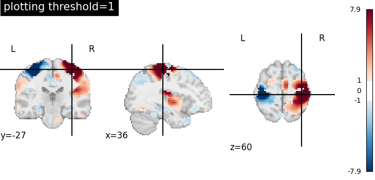
Plotting threshold set to 1

When plotting threshold is set to 1, the values between -1 and 1 are masked in the plot.

plotting.plot_stat_map(
    stat_img,
    threshold=1,
    display_mode="ortho",
    cut_coords=[36, -27, 60],
    title="plotting threshold=1",
)

<nilearn.plotting.displays._slicers.OrthoSlicer object at 0x7f0f33dad2a0>

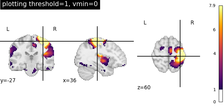
Plotting threshold set to 1 with vmin=0

Setting vmin=0, it is possible to plot only positive image values.

plotting.plot_stat_map(
    stat_img,
    threshold=1,
    cmap="inferno",
    display_mode="ortho",
    cut_coords=[36, -27, 60],
    title="plotting threshold=1, vmin=0",
    vmin=0,
)

<nilearn.plotting.displays._slicers.OrthoSlicer object at 0x7f0f57aae380>

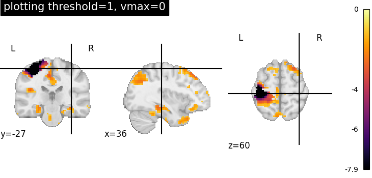
Plotting threshold set to 1 with vmax=0

Setting vmax=0, it is possible to plot only negative image values.

plotting.plot_stat_map(
    stat_img,
    threshold=1,
    cmap="inferno",
    display_mode="ortho",
    cut_coords=[36, -27, 60],
    title="plotting threshold=1, vmax=0",
    vmax=0,
)

<nilearn.plotting.displays._slicers.OrthoSlicer object at 0x7f0f55a6c490>

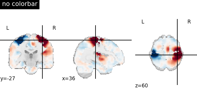
Visualizing without a colorbar on the right side

The argument colorbar should be set to False to show plots without a colorbar on the right side.

plotting.plot_stat_map(
    stat_img,
    display_mode="ortho",
    cut_coords=[36, -27, 60],
    colorbar=False,
    title="no colorbar",
)

<nilearn.plotting.displays._slicers.OrthoSlicer object at 0x7f0f564e3670>

Estimated memory usage: 1037 MB