A introduction tutorial to fMRI decoding

Here is a simple tutorial on decoding with nilearn. It reproduces the Haxby et al.[1] study on a face vs cat discrimination task in a mask of the ventral stream.

This tutorial is meant as an introduction to the various steps of a decoding analysis using Nilearn meta-estimator: Decoder

It is not a minimalistic example, as it strives to be didactic. It is not meant to be copied to analyze new data: many of the steps are unnecessary.

import warnings

warnings.filterwarnings(
    "ignore", message="The provided image has no sform in its header."
)

Retrieve and load the fMRI data from the Haxby study

First download the data

The fetch_haxby function will download the Haxby dataset if not present on the disk, in the nilearn data directory. It can take a while to download about 310 Mo of data from the Internet.

from nilearn import datasets

# By default 2nd subject will be fetched
haxby_dataset = datasets.fetch_haxby()
# 'func' is a list of filenames: one for each subject
fmri_filename = haxby_dataset.func[0]

# print basic information on the dataset
print(f"First subject functional nifti images (4D) are at: {fmri_filename}")

[fetch_haxby] Dataset created in /home/runner/nilearn_data/haxby2001
[fetch_haxby] Downloading data from
https://www.nitrc.org/frs/download.php/7868/mask.nii.gz ...
[fetch_haxby]  ...done. (0 seconds, 0 min)

[fetch_haxby] Downloading data from
http://data.pymvpa.org/datasets/haxby2001/MD5SUMS ...
[fetch_haxby]  ...done. (0 seconds, 0 min)

[fetch_haxby] Downloading data from
http://data.pymvpa.org/datasets/haxby2001/subj2-2010.01.14.tar.gz ...
[fetch_haxby] Downloaded 80625664 of 291168628 bytes (27.7%%,    2.6s remaining)
[fetch_haxby] Downloaded 101081088 of 291168628 bytes (34.7%%,    3.8s
remaining)
[fetch_haxby] Downloaded 113418240 of 291168628 bytes (39.0%%,    4.7s
remaining)
[fetch_haxby] Downloaded 125132800 of 291168628 bytes (43.0%%,    5.3s
remaining)
[fetch_haxby] Downloaded 129761280 of 291168628 bytes (44.6%%,    6.3s
remaining)
[fetch_haxby] Downloaded 135700480 of 291168628 bytes (46.6%%,    6.9s
remaining)
[fetch_haxby] Downloaded 141336576 of 291168628 bytes (48.5%%,    7.5s
remaining)
[fetch_haxby] Downloaded 147750912 of 291168628 bytes (50.7%%,    7.8s
remaining)
[fetch_haxby] Downloaded 156508160 of 291168628 bytes (53.8%%,    7.8s
remaining)
[fetch_haxby] Downloaded 164151296 of 291168628 bytes (56.4%%,    7.8s
remaining)
[fetch_haxby] Downloaded 173948928 of 291168628 bytes (59.7%%,    7.4s
remaining)
[fetch_haxby] Downloaded 185180160 of 291168628 bytes (63.6%%,    6.9s
remaining)
[fetch_haxby] Downloaded 199352320 of 291168628 bytes (68.5%%,    6.0s
remaining)
[fetch_haxby] Downloaded 211271680 of 291168628 bytes (72.6%%,    5.3s
remaining)
[fetch_haxby] Downloaded 217284608 of 291168628 bytes (74.6%%,    5.1s
remaining)
[fetch_haxby] Downloaded 225779712 of 291168628 bytes (77.5%%,    4.7s
remaining)
[fetch_haxby] Downloaded 236290048 of 291168628 bytes (81.2%%,    4.0s
remaining)
[fetch_haxby] Downloaded 246104064 of 291168628 bytes (84.5%%,    3.3s
remaining)
[fetch_haxby] Downloaded 256688128 of 291168628 bytes (88.2%%,    2.6s
remaining)
[fetch_haxby] Downloaded 268066816 of 291168628 bytes (92.1%%,    1.7s
remaining)
[fetch_haxby] Downloaded 279527424 of 291168628 bytes (96.0%%,    0.9s
remaining)
[fetch_haxby]  ...done. (22 seconds, 0 min)

[fetch_haxby] Extracting data from
/home/runner/nilearn_data/haxby2001/9cabe068089e791ef0c5fe930fc20e30/subj2-2010.
01.14.tar.gz...
[fetch_haxby] .. done.

First subject functional nifti images (4D) are at: /home/runner/nilearn_data/haxby2001/subj2/bold.nii.gz

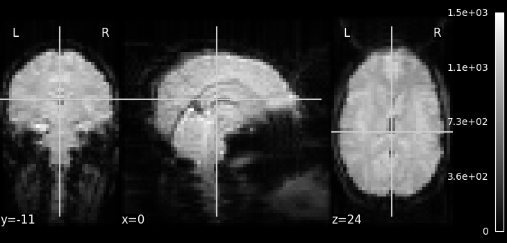
Visualizing the fMRI volume

One way to visualize a fMRI volume is using plot_epi. We will visualize the previously fetched fMRI data from Haxby dataset.

Because fMRI data are 4D (they consist of many 3D EPI images), we cannot plot them directly using plot_epi (which accepts just 3D input). Here we are using mean_img to extract a single 3D EPI image from the fMRI data.

from nilearn.image import mean_img
from nilearn.plotting import plot_epi, plot_roi, show

plot_epi(mean_img(fmri_filename))

show()

Feature extraction: from fMRI volumes to a data matrix

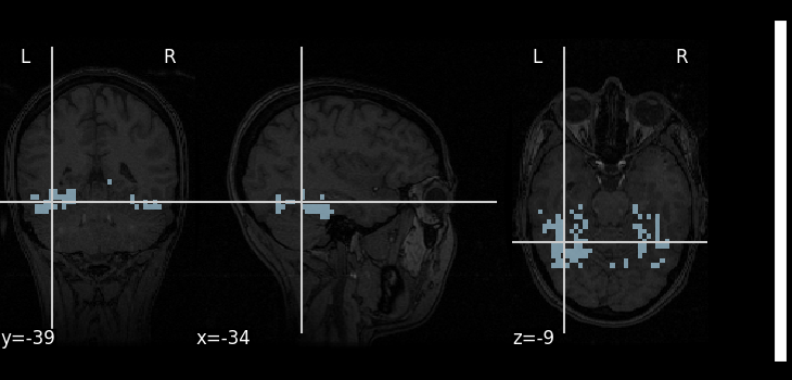
These are some really lovely images, but for machine learning we need matrices to work with the actual data. Fortunately, the Decoder object we will use later on can automatically transform Nifti images into matrices. All we have to do for now is define a mask filename.

A mask of the Ventral Temporal (VT) cortex coming from the Haxby study is available:

mask_filename = haxby_dataset.mask_vt[0]

# Let's visualize it, using the subject's anatomical image as a
# background
plot_roi(mask_filename, bg_img=haxby_dataset.anat[0], cmap="Paired")

show()

Load the behavioral labels

Now that the brain images are converted to a data matrix, we can apply machine-learning to them, for instance to predict the task that the subject was doing. The behavioral labels are stored in a CSV file, separated by spaces.

We use pandas to load them in an array.

import pandas as pd

# Load behavioral information
behavioral = pd.read_csv(haxby_dataset.session_target[0], delimiter=" ")
print(behavioral)

     labels  chunks
0      rest       0
1      rest       0
2      rest       0
3      rest       0
4      rest       0
...     ...     ...
1447   rest      11
1448   rest      11
1449   rest      11
1450   rest      11
1451   rest      11

[1452 rows x 2 columns]

The task was a visual-recognition task, and the labels denote the experimental condition: the type of object that was presented to the subject. This is what we are going to try to predict.

conditions = behavioral["labels"]
print(conditions)

0       rest
1       rest
2       rest
3       rest
4       rest
        ...
1447    rest
1448    rest
1449    rest
1450    rest
1451    rest
Name: labels, Length: 1452, dtype: object

Restrict the analysis to cats and faces

As we can see from the targets above, the experiment contains many conditions. As a consequence, the data is quite big. Not all of this data has an interest to us for decoding, so we will keep only fMRI signals corresponding to faces or cats. We create a mask of the samples belonging to the condition; this mask is then applied to the fMRI data to restrict the classification to the face vs cat discrimination.

The input data will become much smaller (i.e. fMRI signal is shorter):

condition_mask = conditions.isin(["face", "cat"])

Because the data is in one single large 4D image, we need to use index_img to do the split easily.

from nilearn.image import index_img

fmri_niimgs = index_img(fmri_filename, condition_mask)

We apply the same mask to the targets

conditions = conditions[condition_mask]
conditions = conditions.to_numpy()
print(f"{conditions.shape=}")

conditions.shape=(216,)

Decoding with Support Vector Machine

As a decoder, we use a Support Vector Classifier with a linear kernel. We first create it using by using Decoder.

from nilearn.decoding import Decoder

decoder = Decoder(
    estimator="svc",
    mask=mask_filename,
    standardize="zscore_sample",
    screening_percentile=100,
    verbose=1,
)

The decoder object is an object that can be fit (or trained) on data with labels, and then predict labels on data without.

We first fit it on the data

decoder.fit(fmri_niimgs, conditions)

[Decoder.fit] Loading data from <nibabel.nifti1.Nifti1Image object at
0x7f30a2fc69e0>
[Decoder.fit] Loading mask from
'/home/runner/nilearn_data/haxby2001/subj2/mask4_vt.nii.gz'
/home/runner/work/nilearn/nilearn/examples/00_tutorials/plot_decoding_tutorial.py:160: UserWarning: [NiftiMasker.fit] Generation of a mask has been requested (imgs != None) while a mask was given at masker creation. Given mask will be used.
  decoder.fit(fmri_niimgs, conditions)
[Decoder.fit] Resampling mask
[Decoder.fit] Finished fit
[Decoder.fit] Loading data from <nibabel.nifti1.Nifti1Image object at
0x7f30a2fc69e0>
[Decoder.fit] Extracting region signals
[Decoder.fit] Cleaning extracted signals
[Parallel(n_jobs=1)]: Done  10 out of  10 | elapsed:    0.6s finished
[Decoder.fit] Computing image from signals
[Decoder.fit] Computing image from signals
[Decoder.fit] Computing image from signals
[Decoder.fit] Computing image from signals

Decoder(mask='/home/runner/nilearn_data/haxby2001/subj2/mask4_vt.nii.gz',
        screening_percentile=100, standardize='zscore_sample', verbose=1)

In a Jupyter environment, please rerun this cell to show the HTML representation or trust the notebook.
On GitHub, the HTML representation is unable to render, please try loading this page with nbviewer.org.

We can then predict the labels from the data

prediction = decoder.predict(fmri_niimgs)
print(f"{prediction=}")

[Decoder.predict] Loading data from <nibabel.nifti1.Nifti1Image object at
0x7f30a2fc69e0>
[Decoder.predict] Extracting region signals
[Decoder.predict] Cleaning extracted signals
prediction=array(['face', 'face', 'face', 'face', 'face', 'face', 'face', 'face',
       'face', 'cat', 'cat', 'cat', 'cat', 'cat', 'cat', 'cat', 'cat',
       'cat', 'face', 'face', 'face', 'face', 'face', 'face', 'face',
       'face', 'face', 'cat', 'cat', 'cat', 'cat', 'cat', 'cat', 'cat',
       'cat', 'cat', 'face', 'face', 'face', 'face', 'face', 'face',
       'face', 'face', 'face', 'cat', 'cat', 'cat', 'cat', 'cat', 'cat',
       'cat', 'cat', 'cat', 'cat', 'cat', 'cat', 'cat', 'cat', 'cat',
       'cat', 'cat', 'cat', 'face', 'face', 'face', 'face', 'face',
       'face', 'face', 'face', 'face', 'face', 'face', 'face', 'face',
       'face', 'face', 'face', 'face', 'face', 'cat', 'cat', 'cat', 'cat',
       'cat', 'cat', 'cat', 'cat', 'cat', 'cat', 'cat', 'cat', 'cat',
       'cat', 'cat', 'cat', 'cat', 'cat', 'face', 'face', 'face', 'face',
       'face', 'face', 'face', 'face', 'face', 'face', 'face', 'face',
       'face', 'face', 'face', 'face', 'face', 'face', 'cat', 'cat',
       'cat', 'cat', 'cat', 'cat', 'cat', 'cat', 'cat', 'face', 'face',
       'face', 'face', 'face', 'face', 'face', 'face', 'face', 'cat',
       'cat', 'cat', 'cat', 'cat', 'cat', 'cat', 'cat', 'cat', 'face',
       'face', 'face', 'face', 'face', 'face', 'face', 'face', 'face',
       'cat', 'cat', 'cat', 'cat', 'cat', 'cat', 'cat', 'cat', 'cat',
       'face', 'face', 'face', 'face', 'face', 'face', 'face', 'face',
       'face', 'cat', 'cat', 'cat', 'cat', 'cat', 'cat', 'cat', 'cat',
       'cat', 'cat', 'cat', 'cat', 'cat', 'cat', 'cat', 'cat', 'cat',
       'cat', 'face', 'face', 'face', 'face', 'face', 'face', 'face',
       'face', 'face', 'face', 'face', 'face', 'face', 'face', 'face',
       'face', 'face', 'face', 'cat', 'cat', 'cat', 'cat', 'cat', 'cat',
       'cat', 'cat', 'cat'], dtype='<U4')

Note that for this classification task both classes contain the same number of samples (the problem is balanced). Then, we can use accuracy to measure the performance of the decoder. This is done by defining accuracy as the scoring. Let’s measure the prediction accuracy:

print((prediction == conditions).sum() / float(len(conditions)))

1.0

This prediction accuracy score is meaningless. Why?

Measuring prediction scores using cross-validation

The proper way to measure error rates or prediction accuracy is via cross-validation: leaving out some data and testing on it.

Manually leaving out data

Let’s leave out the 30 last data points during training, and test the prediction on these 30 last points:

fmri_niimgs_train = index_img(fmri_niimgs, slice(0, -30))
fmri_niimgs_test = index_img(fmri_niimgs, slice(-30, None))
conditions_train = conditions[:-30]
conditions_test = conditions[-30:]

decoder = Decoder(
    estimator="svc",
    mask=mask_filename,
    standardize="zscore_sample",
    screening_percentile=100,
    verbose=1,
)
decoder.fit(fmri_niimgs_train, conditions_train)

prediction = decoder.predict(fmri_niimgs_test)

# The prediction accuracy is calculated on the test data: this is the accuracy
# of our model on examples it hasn't seen to examine how well the model perform
# in general.

predicton_accuracy = (prediction == conditions_test).sum() / float(
    len(conditions_test)
)
print(f"Prediction Accuracy: {predicton_accuracy:.3f}")

[Decoder.fit] Loading data from <nibabel.nifti1.Nifti1Image object at
0x7f30a2a2b0d0>
[Decoder.fit] Loading mask from
'/home/runner/nilearn_data/haxby2001/subj2/mask4_vt.nii.gz'
/home/runner/work/nilearn/nilearn/examples/00_tutorials/plot_decoding_tutorial.py:202: UserWarning: [NiftiMasker.fit] Generation of a mask has been requested (imgs != None) while a mask was given at masker creation. Given mask will be used.
  decoder.fit(fmri_niimgs_train, conditions_train)
[Decoder.fit] Resampling mask
[Decoder.fit] Finished fit
[Decoder.fit] Loading data from <nibabel.nifti1.Nifti1Image object at
0x7f30a2a2b0d0>
[Decoder.fit] Extracting region signals
[Decoder.fit] Cleaning extracted signals
[Parallel(n_jobs=1)]: Done  10 out of  10 | elapsed:    0.6s finished
[Decoder.fit] Computing image from signals
[Decoder.fit] Computing image from signals
[Decoder.fit] Computing image from signals
[Decoder.fit] Computing image from signals
[Decoder.predict] Loading data from <nibabel.nifti1.Nifti1Image object at
0x7f30a2a2a5f0>
[Decoder.predict] Extracting region signals
[Decoder.predict] Cleaning extracted signals
Prediction Accuracy: 0.767

Implementing a KFold loop

We can manually split the data in train and test set repetitively in a KFold strategy by importing scikit-learn’s object:

from sklearn.model_selection import KFold

cv = KFold(n_splits=5)

for fold, (train, test) in enumerate(cv.split(conditions), start=1):
    decoder = Decoder(
        estimator="svc",
        mask=mask_filename,
        standardize="zscore_sample",
        screening_percentile=100,
        verbose=1,
    )
    decoder.fit(index_img(fmri_niimgs, train), conditions[train])
    prediction = decoder.predict(index_img(fmri_niimgs, test))
    predicton_accuracy = (prediction == conditions[test]).sum() / float(
        len(conditions[test])
    )
    print(
        f"CV Fold {fold:01d} | Prediction Accuracy: {predicton_accuracy:.3f}"
    )

[Decoder.fit] Loading data from <nibabel.nifti1.Nifti1Image object at
0x7f30a2a2b100>
[Decoder.fit] Loading mask from
'/home/runner/nilearn_data/haxby2001/subj2/mask4_vt.nii.gz'
/home/runner/work/nilearn/nilearn/examples/00_tutorials/plot_decoding_tutorial.py:233: UserWarning: [NiftiMasker.fit] Generation of a mask has been requested (imgs != None) while a mask was given at masker creation. Given mask will be used.
  decoder.fit(index_img(fmri_niimgs, train), conditions[train])
[Decoder.fit] Resampling mask
[Decoder.fit] Finished fit
[Decoder.fit] Loading data from <nibabel.nifti1.Nifti1Image object at
0x7f30a2a2b100>
[Decoder.fit] Extracting region signals
[Decoder.fit] Cleaning extracted signals
[Parallel(n_jobs=1)]: Done  10 out of  10 | elapsed:    0.4s finished
[Decoder.fit] Computing image from signals
[Decoder.fit] Computing image from signals
[Decoder.fit] Computing image from signals
[Decoder.fit] Computing image from signals
[Decoder.predict] Loading data from <nibabel.nifti1.Nifti1Image object at
0x7f30c3527ee0>
[Decoder.predict] Extracting region signals
[Decoder.predict] Cleaning extracted signals
CV Fold 1 | Prediction Accuracy: 0.886
[Decoder.fit] Loading data from <nibabel.nifti1.Nifti1Image object at
0x7f30a2a28340>
[Decoder.fit] Loading mask from
'/home/runner/nilearn_data/haxby2001/subj2/mask4_vt.nii.gz'
/home/runner/work/nilearn/nilearn/examples/00_tutorials/plot_decoding_tutorial.py:233: UserWarning: [NiftiMasker.fit] Generation of a mask has been requested (imgs != None) while a mask was given at masker creation. Given mask will be used.
  decoder.fit(index_img(fmri_niimgs, train), conditions[train])
[Decoder.fit] Resampling mask
[Decoder.fit] Finished fit
[Decoder.fit] Loading data from <nibabel.nifti1.Nifti1Image object at
0x7f30a2a28340>
[Decoder.fit] Extracting region signals
[Decoder.fit] Cleaning extracted signals
[Parallel(n_jobs=1)]: Done  10 out of  10 | elapsed:    0.6s finished
[Decoder.fit] Computing image from signals
[Decoder.fit] Computing image from signals
[Decoder.fit] Computing image from signals
[Decoder.fit] Computing image from signals
[Decoder.predict] Loading data from <nibabel.nifti1.Nifti1Image object at
0x7f30c3527ee0>
[Decoder.predict] Extracting region signals
[Decoder.predict] Cleaning extracted signals
CV Fold 2 | Prediction Accuracy: 0.767
[Decoder.fit] Loading data from <nibabel.nifti1.Nifti1Image object at
0x7f30a2a2a1d0>
[Decoder.fit] Loading mask from
'/home/runner/nilearn_data/haxby2001/subj2/mask4_vt.nii.gz'
/home/runner/work/nilearn/nilearn/examples/00_tutorials/plot_decoding_tutorial.py:233: UserWarning: [NiftiMasker.fit] Generation of a mask has been requested (imgs != None) while a mask was given at masker creation. Given mask will be used.
  decoder.fit(index_img(fmri_niimgs, train), conditions[train])
[Decoder.fit] Resampling mask
[Decoder.fit] Finished fit
[Decoder.fit] Loading data from <nibabel.nifti1.Nifti1Image object at
0x7f30a2a2a1d0>
[Decoder.fit] Extracting region signals
[Decoder.fit] Cleaning extracted signals
[Parallel(n_jobs=1)]: Done  10 out of  10 | elapsed:    0.5s finished
[Decoder.fit] Computing image from signals
[Decoder.fit] Computing image from signals
[Decoder.fit] Computing image from signals
[Decoder.fit] Computing image from signals
[Decoder.predict] Loading data from <nibabel.nifti1.Nifti1Image object at
0x7f30c3527ee0>
[Decoder.predict] Extracting region signals
[Decoder.predict] Cleaning extracted signals
CV Fold 3 | Prediction Accuracy: 0.767
[Decoder.fit] Loading data from <nibabel.nifti1.Nifti1Image object at
0x7f30a2a294b0>
[Decoder.fit] Loading mask from
'/home/runner/nilearn_data/haxby2001/subj2/mask4_vt.nii.gz'
/home/runner/work/nilearn/nilearn/examples/00_tutorials/plot_decoding_tutorial.py:233: UserWarning: [NiftiMasker.fit] Generation of a mask has been requested (imgs != None) while a mask was given at masker creation. Given mask will be used.
  decoder.fit(index_img(fmri_niimgs, train), conditions[train])
[Decoder.fit] Resampling mask
[Decoder.fit] Finished fit
[Decoder.fit] Loading data from <nibabel.nifti1.Nifti1Image object at
0x7f30a2a294b0>
[Decoder.fit] Extracting region signals
[Decoder.fit] Cleaning extracted signals
[Parallel(n_jobs=1)]: Done  10 out of  10 | elapsed:    0.5s finished
[Decoder.fit] Computing image from signals
[Decoder.fit] Computing image from signals
[Decoder.fit] Computing image from signals
[Decoder.fit] Computing image from signals
[Decoder.predict] Loading data from <nibabel.nifti1.Nifti1Image object at
0x7f30c3526920>
[Decoder.predict] Extracting region signals
[Decoder.predict] Cleaning extracted signals
CV Fold 4 | Prediction Accuracy: 0.698
[Decoder.fit] Loading data from <nibabel.nifti1.Nifti1Image object at
0x7f30a2a289d0>
[Decoder.fit] Loading mask from
'/home/runner/nilearn_data/haxby2001/subj2/mask4_vt.nii.gz'
/home/runner/work/nilearn/nilearn/examples/00_tutorials/plot_decoding_tutorial.py:233: UserWarning: [NiftiMasker.fit] Generation of a mask has been requested (imgs != None) while a mask was given at masker creation. Given mask will be used.
  decoder.fit(index_img(fmri_niimgs, train), conditions[train])
[Decoder.fit] Resampling mask
[Decoder.fit] Finished fit
[Decoder.fit] Loading data from <nibabel.nifti1.Nifti1Image object at
0x7f30a2a289d0>
[Decoder.fit] Extracting region signals
[Decoder.fit] Cleaning extracted signals
[Parallel(n_jobs=1)]: Done  10 out of  10 | elapsed:    0.5s finished
[Decoder.fit] Computing image from signals
[Decoder.fit] Computing image from signals
[Decoder.fit] Computing image from signals
[Decoder.fit] Computing image from signals
[Decoder.predict] Loading data from <nibabel.nifti1.Nifti1Image object at
0x7f30c3526920>
[Decoder.predict] Extracting region signals
[Decoder.predict] Cleaning extracted signals
CV Fold 5 | Prediction Accuracy: 0.744

Cross-validation with the decoder

The decoder also implements a cross-validation loop by default and returns an array of shape (cross-validation parameters, n_folds). We can use accuracy score to measure its performance by defining accuracy as the scoring parameter.

n_folds = 5
decoder = Decoder(
    estimator="svc",
    mask=mask_filename,
    standardize="zscore_sample",
    cv=n_folds,
    scoring="accuracy",
    screening_percentile=100,
    verbose=1,
)
decoder.fit(fmri_niimgs, conditions)

[Decoder.fit] Loading data from <nibabel.nifti1.Nifti1Image object at
0x7f30a2fc69e0>
[Decoder.fit] Loading mask from
'/home/runner/nilearn_data/haxby2001/subj2/mask4_vt.nii.gz'
/home/runner/work/nilearn/nilearn/examples/00_tutorials/plot_decoding_tutorial.py:260: UserWarning: [NiftiMasker.fit] Generation of a mask has been requested (imgs != None) while a mask was given at masker creation. Given mask will be used.
  decoder.fit(fmri_niimgs, conditions)
[Decoder.fit] Resampling mask
[Decoder.fit] Finished fit
[Decoder.fit] Loading data from <nibabel.nifti1.Nifti1Image object at
0x7f30a2fc69e0>
[Decoder.fit] Extracting region signals
[Decoder.fit] Cleaning extracted signals
[Parallel(n_jobs=1)]: Done   5 out of   5 | elapsed:    0.3s finished
[Decoder.fit] Computing image from signals
[Decoder.fit] Computing image from signals
[Decoder.fit] Computing image from signals
[Decoder.fit] Computing image from signals

Decoder(cv=5, mask='/home/runner/nilearn_data/haxby2001/subj2/mask4_vt.nii.gz',
        scoring='accuracy', screening_percentile=100,
        standardize='zscore_sample', verbose=1)

In a Jupyter environment, please rerun this cell to show the HTML representation or trust the notebook.
On GitHub, the HTML representation is unable to render, please try loading this page with nbviewer.org.

Cross-validation pipeline can also be implemented manually. More details can be found on scikit-learn website.

Then we can check the best performing parameters per fold.

print(decoder.cv_params_["face"])

{'C': [np.float64(100.0), np.float64(100.0), np.float64(100.0), np.float64(100.0), np.float64(100.0)]}

Note

We can speed things up to use all the CPUs of our computer with the n_jobs parameter.

The best way to do cross-validation is to respect the structure of the experiment, for instance by leaving out full runs of acquisition.

The number of the run is stored in the CSV file giving the behavioral data. We have to apply our run mask, to select only cats and faces.

run_label = behavioral["chunks"][condition_mask]

The fMRI data is acquired by runs, and the noise is autocorrelated in a given run. Hence, it is better to predict across runs when doing cross-validation. To leave a run out, pass the cross-validator object to the cv parameter of decoder.

from sklearn.model_selection import LeaveOneGroupOut

cv = LeaveOneGroupOut()

decoder = Decoder(
    estimator="svc",
    mask=mask_filename,
    standardize="zscore_sample",
    cv=cv,
    screening_percentile=100,
    verbose=1,
)
decoder.fit(fmri_niimgs, conditions, groups=run_label)

print(f"{decoder.cv_scores_=}")

[Decoder.fit] Loading data from <nibabel.nifti1.Nifti1Image object at
0x7f30a2fc69e0>
[Decoder.fit] Loading mask from
'/home/runner/nilearn_data/haxby2001/subj2/mask4_vt.nii.gz'
/home/runner/work/nilearn/nilearn/examples/00_tutorials/plot_decoding_tutorial.py:302: UserWarning: [NiftiMasker.fit] Generation of a mask has been requested (imgs != None) while a mask was given at masker creation. Given mask will be used.
  decoder.fit(fmri_niimgs, conditions, groups=run_label)
[Decoder.fit] Resampling mask
[Decoder.fit] Finished fit
[Decoder.fit] Loading data from <nibabel.nifti1.Nifti1Image object at
0x7f30a2fc69e0>
[Decoder.fit] Extracting region signals
[Decoder.fit] Cleaning extracted signals
[Parallel(n_jobs=1)]: Done  12 out of  12 | elapsed:    0.8s finished
[Decoder.fit] Computing image from signals
[Decoder.fit] Computing image from signals
[Decoder.fit] Computing image from signals
[Decoder.fit] Computing image from signals
decoder.cv_scores_={np.str_('cat'): [1.0, 1.0, 1.0, 1.0, 0.9629629629629629, 0.8518518518518519, 0.9753086419753086, 0.40740740740740744, 0.9876543209876543, 1.0, 0.9259259259259259, 0.8765432098765432], np.str_('face'): [1.0, 1.0, 1.0, 1.0, 0.9629629629629629, 0.8518518518518519, 0.9753086419753086, 0.40740740740740744, 0.9876543209876543, 1.0, 0.9259259259259259, 0.8765432098765432]}

Inspecting the model weights

Finally, it may be useful to inspect and display the model weights.

Turning the weights into a nifti image

We retrieve the SVC discriminating weights

coef_ = decoder.coef_
print(f"{coef_=}")

coef_=array([[-3.89376784e-02, -1.87167024e-02, -3.23027450e-02,
        -2.88746517e-02,  4.18696469e-02,  1.10744242e-02,
         1.69997895e-02, -5.50956812e-02, -1.94204166e-02,
        -3.51225128e-02,  1.08511915e-02, -1.28797537e-02,
        -1.54677563e-02, -3.78907351e-02, -3.69170867e-02,
         2.28086779e-02,  6.56427594e-03, -7.65759439e-03,
         1.67106564e-02, -8.02156650e-03,  5.29514633e-02,
        -8.17596074e-02, -6.36992254e-02,  2.41325128e-02,
         4.59875031e-02, -2.22602734e-02, -1.77309591e-02,
         2.22196387e-02, -9.53198269e-03,  5.76046111e-02,
         2.14299576e-02, -9.14225721e-02,  4.03670838e-03,
        -2.89274656e-02, -3.89029396e-02, -3.35115812e-02,
         2.21394600e-03,  8.73137535e-03, -3.37415969e-02,
        -2.41273486e-02, -6.81648526e-02,  1.65405916e-02,
         2.70784914e-02, -6.56857667e-03, -1.21662920e-02,
         5.47675488e-02,  8.13260591e-03,  3.60956193e-02,
        -1.52762484e-02,  7.02913408e-02,  1.28107452e-03,
         2.08010053e-02, -4.09958163e-03,  3.72430455e-02,
        -3.77396055e-02, -1.03858258e-02, -2.38236930e-02,
        -5.48881404e-02,  4.43028798e-02, -1.47419286e-01,
        -2.34044527e-02,  1.87115223e-02,  6.65860904e-02,
        -9.07602120e-02, -1.22035172e-02, -2.95627978e-03,
         3.22092401e-02, -3.04053455e-02,  6.15346355e-02,
         1.12248612e-02,  1.93776721e-02, -1.30543022e-02,
         4.42975742e-02, -2.23065490e-02,  6.88148535e-02,
         1.69390499e-02,  1.78947322e-02,  1.00277303e-02,
         2.99186755e-02, -2.52169254e-02,  1.06154557e-02,
        -6.31952325e-03,  2.21508262e-03, -2.23348688e-02,
         1.42560949e-02, -1.53123536e-02, -1.98226755e-02,
        -4.32638490e-02, -4.55124093e-02,  3.41589325e-02,
        -2.79199355e-02, -2.80912363e-02, -3.70160501e-02,
        -5.71450869e-02, -6.98950572e-02,  3.20161044e-03,
        -8.35432812e-03, -3.37625457e-02,  3.04261878e-02,
         8.68462151e-03,  6.19393933e-03,  5.94178209e-02,
         9.07298029e-03, -1.48932250e-02,  1.43559820e-02,
        -1.09027358e-02,  2.67698473e-02,  4.73788393e-02,
        -2.96433232e-02,  3.09420891e-02,  1.57927296e-02,
        -3.16719717e-02, -4.00107065e-02, -5.40260563e-02,
         2.82611038e-02, -1.12100352e-02, -5.45403087e-02,
         6.32178093e-02, -1.49996813e-02,  2.47548350e-03,
        -4.56645115e-02, -1.83881961e-02,  1.19957262e-02,
        -3.72173617e-02, -2.25518631e-03,  4.58653677e-02,
         4.79164136e-02,  2.51823295e-03, -4.31721187e-02,
        -5.35329000e-03,  5.76993605e-02,  7.40826182e-03,
        -3.20589549e-02,  4.35701059e-03,  1.68303059e-02,
        -2.92569881e-02, -2.24495566e-03, -8.30218254e-03,
        -1.00013848e-02,  2.17135085e-02, -1.92626439e-03,
        -1.33222562e-02, -2.80298557e-02, -1.75292616e-02,
        -9.17805143e-03, -7.09943043e-03, -1.43034312e-02,
         5.06832851e-02, -1.84814291e-02, -4.71510900e-02,
         1.72568091e-02, -4.76642901e-02, -9.09257707e-04,
         4.00770435e-02,  7.53994497e-02,  7.25616319e-03,
         4.82603924e-02,  4.50555855e-02,  3.61203786e-02,
        -8.16488973e-03,  1.95405323e-02,  3.57884701e-02,
         4.89306317e-02,  3.82973071e-02,  6.23921930e-02,
         6.13673059e-02, -1.68751875e-02,  1.66514433e-02,
         3.35524345e-02, -1.80214164e-02,  4.46409790e-02,
        -3.53245562e-02, -3.67293158e-02, -4.62259250e-03,
         4.86832207e-02,  3.39666324e-02,  6.21703022e-03,
         1.73610999e-02,  2.01697095e-02,  2.17096021e-02,
         2.91414537e-02,  2.37776993e-02,  4.84697460e-02,
        -9.22625464e-03, -2.82637566e-02, -2.13780685e-02,
         1.80780139e-03,  4.79690231e-02, -9.78894271e-03,
         1.11431545e-02, -1.65020151e-02, -2.89089254e-02,
         2.42849583e-02, -1.22347326e-02, -2.92870573e-02,
        -2.89845916e-02, -3.39532821e-02, -3.65288266e-03,
         2.65322387e-02,  4.58040244e-02, -5.93381008e-02,
        -2.13629782e-02, -3.09404873e-02,  5.50177505e-02,
        -3.38817353e-02,  6.12630910e-03,  1.41484367e-02,
         1.10217408e-02,  5.33810502e-02, -2.12339623e-02,
         6.37419827e-03, -1.13075881e-02, -2.64227317e-02,
        -2.22398945e-02, -5.31920762e-02, -3.98654172e-02,
        -1.29727566e-01, -3.28090570e-02, -2.89710211e-02,
        -9.13472648e-03, -7.28725478e-03, -3.71051650e-02,
        -6.34907087e-02,  2.04396696e-03, -8.26795632e-02,
        -6.71216548e-02, -2.29125975e-03, -2.33450771e-02,
         1.77913344e-02, -8.74665871e-02, -2.76491866e-03,
        -4.38275342e-02, -1.28050054e-02,  2.78033464e-02,
        -4.32696436e-02, -3.22689143e-02, -2.28028600e-02,
        -2.57413951e-02,  2.03623726e-02, -9.90248070e-03,
        -3.15035027e-02, -1.81419995e-02, -1.12292462e-03,
        -4.17433458e-02, -6.23479579e-02,  2.54745277e-04,
        -6.73679264e-02,  6.53964606e-02,  1.06522492e-02,
         2.21985517e-02, -1.98727017e-02, -1.85520222e-02,
         4.05702232e-02, -3.02838061e-02, -8.10051101e-02,
        -7.42458860e-02, -4.93850754e-02, -1.01769423e-02,
         1.09409859e-02, -4.49253737e-02,  2.92749554e-02,
         7.05312786e-03,  5.07553398e-03, -4.84042061e-03,
         2.48719241e-03,  3.00654455e-02, -2.63100147e-03,
         4.64686199e-03,  7.90209355e-02,  1.04858038e-02,
         1.68079537e-02, -4.36718492e-02, -1.08854463e-02,
         2.10241605e-02, -4.41964323e-02,  3.16491276e-03,
         6.98672061e-02,  8.61630771e-02,  4.96233386e-02,
         6.03889598e-03,  5.56494339e-02, -2.98919432e-02,
         4.13043711e-03, -3.21953397e-02, -3.14991498e-02,
        -5.31277184e-02,  2.67255450e-02,  3.14427984e-02,
         6.67111722e-03, -1.28703377e-02,  2.20150499e-02,
         5.68523120e-02,  2.25602473e-02, -2.04617249e-02,
         5.10341400e-03,  2.85357342e-02, -1.81665500e-02,
        -8.48452742e-03, -3.18824041e-02, -1.18500540e-02,
        -4.10845023e-02,  3.11780533e-02,  9.63467926e-03,
        -8.25913608e-03, -3.12228797e-02,  8.57659322e-03,
        -9.70205341e-03,  1.32374563e-02,  4.06447054e-02,
         8.23367760e-03, -3.27356276e-02, -4.33864892e-03,
        -1.75530738e-02,  6.88833922e-03,  3.45132274e-02,
         7.03298417e-02,  2.16785027e-02,  5.32222430e-03,
         8.17562670e-02,  6.40063432e-02, -2.31133294e-03,
        -1.17555969e-02,  1.75889107e-01,  3.18129342e-02,
        -3.15887119e-02,  3.34027907e-02,  2.22783904e-02,
         1.00229602e-02, -4.74914386e-02, -2.12759013e-02,
        -3.98717445e-02, -6.04067339e-02, -4.65059907e-02,
         1.03004015e-02, -3.05634290e-04,  1.80742885e-02,
        -1.75452794e-02, -8.72590901e-02,  1.00662472e-01,
         4.46103998e-03,  7.46870782e-02, -6.13410063e-02,
         2.81704993e-02, -1.40977259e-02,  3.14637628e-02,
        -1.63833904e-02,  3.66533114e-02, -5.15678912e-03,
         1.45094238e-02,  6.35865946e-02,  2.34599201e-02,
         8.81060263e-02,  6.15344047e-02, -1.39361184e-02,
         2.07246295e-02, -3.15477310e-03,  5.15425799e-02,
        -2.88767805e-02,  1.60262554e-02,  2.09702644e-02,
        -3.29173417e-02, -2.59463483e-02, -5.60400966e-02,
        -3.64629066e-02,  1.12882241e-02,  2.17267721e-02,
        -1.51637011e-02, -7.82896239e-03,  2.42548919e-02,
         9.47013746e-02, -2.63033478e-02,  1.17282688e-04,
        -5.24185288e-03,  4.17987165e-02,  8.85681063e-02,
         6.23645937e-03,  1.86599557e-02,  1.54628862e-02,
         3.50536538e-03,  6.20597572e-03, -1.19790193e-02,
         1.59526160e-02,  7.12138968e-03, -8.93192416e-02,
        -3.54346644e-03,  1.23477670e-02,  3.03927938e-02,
        -2.37293881e-02, -3.82793044e-02, -4.98744109e-02,
         4.66896351e-02, -1.23291954e-02, -1.10332250e-02,
         2.18106731e-02,  2.18720167e-02,  2.63537724e-02,
         1.05280826e-02,  1.84617882e-02,  8.36027156e-04,
        -6.65215848e-03,  3.49398015e-02,  1.49353942e-02,
        -1.11599656e-02,  6.69109594e-03, -2.00058718e-02,
        -3.99014665e-02,  3.01872539e-02, -1.09867310e-02,
        -4.11779618e-02,  2.72052450e-02,  1.16426452e-02,
        -1.55501773e-02,  3.27700605e-02,  3.95493420e-02,
         8.48743641e-03,  2.19936986e-02, -9.88671612e-03,
        -3.61421611e-02, -4.77020548e-02,  1.90072573e-02,
        -5.58286520e-02, -3.31739367e-02, -2.24912988e-02,
        -3.36176498e-02, -4.07357452e-02,  1.08861926e-02,
         1.12812613e-02,  7.63143795e-02,  4.04806939e-03,
         3.07013611e-02,  2.89177758e-02,  4.71607708e-03,
         5.13383889e-02, -4.10363924e-02,  1.23259199e-03,
        -2.50402468e-02,  5.85904765e-02, -1.04965598e-01,
        -4.41704198e-02,  1.18518961e-02, -5.83203241e-02,
        -4.82245347e-02,  9.17683449e-03,  1.03260196e-02,
        -5.09179542e-03, -3.23391676e-02, -3.19384386e-02,
        -1.53770251e-02, -5.21212972e-02,  1.55620419e-02,
         2.93484347e-02, -1.92528128e-02,  1.76695372e-02,
         2.67992361e-02,  5.76552598e-02, -1.38162742e-02,
         2.60398776e-02,  1.50401048e-02,  1.27425007e-02,
        -2.29244622e-02, -1.06665617e-02,  9.81935178e-03,
        -4.77512412e-02,  1.64242712e-02]])

It’s a numpy array with only one coefficient per voxel:

print(f"{coef_.shape=}")

coef_.shape=(1, 464)

To get the Nifti image of these coefficients, we only need retrieve the coef_img_ in the decoder and select the class

coef_img = decoder.coef_img_["face"]

coef_img is now a NiftiImage. We can save the coefficients as a nii.gz file:

from pathlib import Path

output_dir = Path.cwd() / "results" / "plot_decoding_tutorial"
output_dir.mkdir(exist_ok=True, parents=True)
print(f"Output will be saved to: {output_dir}")
decoder.coef_img_["face"].to_filename(output_dir / "haxby_svc_weights.nii.gz")

Output will be saved to: /home/runner/work/nilearn/nilearn/examples/00_tutorials/results/plot_decoding_tutorial

Plotting the SVM weights

We can plot the weights, using the subject’s anatomical as a background

from nilearn.plotting import view_img

view_img(
    decoder.coef_img_["face"],
    bg_img=haxby_dataset.anat[0],
    title="SVM weights",
    dim=-1,
)

/home/runner/work/nilearn/nilearn/.tox/doc/lib/python3.10/site-packages/numpy/_core/fromnumeric.py:868: UserWarning: Warning: 'partition' will ignore the 'mask' of the MaskedArray.
  a.partition(kth, axis=axis, kind=kind, order=order)

What is the chance level accuracy?

Does the model above perform better than chance? To answer this question, we measure a score at random using simple strategies that are implemented in the Decoder object. This is useful to inspect the decoding performance by comparing to a score at chance.

Let’s define a object with Dummy estimator replacing ‘svc’ for classification setting. This object initializes estimator with default dummy strategy.

dummy_decoder = Decoder(
    estimator="dummy_classifier",
    mask=mask_filename,
    cv=cv,
    standardize="zscore_sample",
    screening_percentile=100,
    verbose=1,
)
dummy_decoder.fit(fmri_niimgs, conditions, groups=run_label)

# Now, we can compare these scores by simply taking a mean over folds
print(f"{dummy_decoder.cv_scores_=}")

[Decoder.fit] Loading data from <nibabel.nifti1.Nifti1Image object at
0x7f30a2fc69e0>
[Decoder.fit] Loading mask from
'/home/runner/nilearn_data/haxby2001/subj2/mask4_vt.nii.gz'
/home/runner/work/nilearn/nilearn/examples/00_tutorials/plot_decoding_tutorial.py:373: UserWarning: [NiftiMasker.fit] Generation of a mask has been requested (imgs != None) while a mask was given at masker creation. Given mask will be used.
  dummy_decoder.fit(fmri_niimgs, conditions, groups=run_label)
[Decoder.fit] Resampling mask
[Decoder.fit] Finished fit
[Decoder.fit] Loading data from <nibabel.nifti1.Nifti1Image object at
0x7f30a2fc69e0>
[Decoder.fit] Extracting region signals
[Decoder.fit] Cleaning extracted signals
[Parallel(n_jobs=1)]: Done  12 out of  12 | elapsed:    0.0s finished
dummy_decoder.cv_scores_={np.str_('cat'): [0.38888888888888895, 0.38888888888888895, 0.38888888888888895, 0.6111111111111112, 0.38888888888888895, 0.6111111111111112, 0.38888888888888895, 0.38888888888888895, 0.38888888888888895, 0.38888888888888895, 0.6111111111111112, 0.38888888888888895], np.str_('face'): [0.38888888888888895, 0.38888888888888895, 0.38888888888888895, 0.6111111111111112, 0.38888888888888895, 0.6111111111111112, 0.38888888888888895, 0.38888888888888895, 0.38888888888888895, 0.38888888888888895, 0.6111111111111112, 0.38888888888888895]}

References

[1]

James V. Haxby, M. Ida Gobbini, Maura L. Furey, Alumit Ishai, Jennifer L. Schouten, and Pietro Pietrini. Distributed and overlapping representations of faces and objects in ventral temporal cortex. Science, 293(5539):2425–2430, 2001. doi:10.1126/science.1063736.

See also

• The section of the documentation on decoding

• Understanding Decoder For a more in-depth understanding of the Decoder

• Decoding with ANOVA + SVM: face vs house in the Haxby dataset For decoding without a precomputed mask

• FREM: fast ensembling of regularized models for robust decoding

• SpaceNet: decoding with spatial structure for better maps

---

Estimated memory usage: 1019 MB