Seed-based connectivity on the surface

In this example we compute the functional connectivity of a seed region to all other cortical nodes in the same hemisphere using Pearson product-moment correlation coefficient.

This example use the resting state time series of a single subject’s left hemisphere the NKI enhanced surface dataset.

The Destrieux atlas in fsaverage5 space is used to select a seed region in the posterior cingulate cortex.

The plot_surf_stat_map function is used to plot the resulting statistical map on the pial surface.

See also

for a similar example but using volumetric input data.

See Plotting brain images for more details on plotting tools.

See the dataset description for more information on the data used in this example.

Retrieving the data

from nilearn.datasets import (
    fetch_atlas_surf_destrieux,
    load_fsaverage,
    load_fsaverage_data,
    load_nki,
)
from nilearn.surface import SurfaceImage

# The nki list contains a SurfaceImage instance
# with fsaverage_meshes pial meshes
# for each subject.
fsaverage_mesh = "fsaverage5"
surf_img_nki = load_nki(
    mesh=fsaverage_mesh,
    mesh_type="pial",
    n_subjects=1,
)[0]


# Get fsaverage meshes and Destrieux parcellation
fsaverage_meshes = load_fsaverage(mesh=fsaverage_mesh)
destrieux = fetch_atlas_surf_destrieux()

# Create a surface image instance
# with the Destrieux parcellation
destrieux_atlas = SurfaceImage(
    mesh=fsaverage_meshes["pial"],
    data={
        "left": destrieux.map_left,
        "right": destrieux.map_right,
    },
)

# The fsaverage meshes contains FileMesh objects:
print(f"{fsaverage_meshes['pial'].parts['left']=}")

# The fsaverage data contains SurfaceImage instances with meshes and data
fsaverage_sulcal = load_fsaverage_data(data_type="sulcal")
print(f"{fsaverage_sulcal=}")
print(f"{fsaverage_sulcal.mesh=}")
print(f"{fsaverage_sulcal.data=}")

[get_dataset_dir] Dataset found in
/home/runner/nilearn_data/nki_enhanced_surface
[load_nki] Loading subject 1 of 1.
[get_dataset_dir] Dataset found in /home/runner/nilearn_data/destrieux_surface
/home/runner/work/nilearn/nilearn/examples/01_plotting/plot_surf_stat_map.py:56: UserWarning:
The following regions are present in the atlas look-up table,
but missing from the atlas image:

 index    name
     0 Unknown

  destrieux = fetch_atlas_surf_destrieux()
/home/runner/work/nilearn/nilearn/examples/01_plotting/plot_surf_stat_map.py:56: UserWarning:
The following regions are present in the atlas look-up table,
but missing from the atlas image:

 index    name
     0 Unknown

  destrieux = fetch_atlas_surf_destrieux()
fsaverage_meshes['pial'].parts['left']=<FileMesh with 10242 vertices and 20480 faces.>
fsaverage_sulcal=<SurfaceImage (20484,)>
fsaverage_sulcal.mesh=<nilearn.surface.surface.PolyMesh object at 0x7fc1ee7c4910>
fsaverage_sulcal.data=<PolyData (20484,)>

Extracting the seed time series with masker

We do this using the SurfaceLabelsMasker.

import numpy as np

from nilearn.maskers import SurfaceLabelsMasker

# Extract seed region via label
name_seed_region = "G_cingul-Post-dorsal"
label_seed_region = destrieux.labels.index(name_seed_region)

# Here we create a surface mask image
# that has False for all vertices
# except for those of the seed region.
mask_data = {}
for hemi, data in destrieux_atlas.data.parts.items():
    seed_vertices = data == label_seed_region
    mask_data[hemi] = seed_vertices

pcc_mask = SurfaceImage(
    mesh=destrieux_atlas.mesh,
    data=mask_data,
)

masker = SurfaceLabelsMasker(labels_img=pcc_mask).fit()
seed_timeseries = masker.transform(surf_img_nki).squeeze()

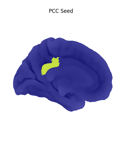
Display ROI on surface

Before we go further, let’s make sure we have selected the right regions.

from nilearn.plotting import plot_surf_roi, show

# For this example we will only show
# and compute results
# on the left hemisphere
# for the sake of speed.
hemisphere = "left"

plot_surf_roi(
    roi_map=pcc_mask,
    hemi=hemisphere,
    view="medial",
    bg_map=fsaverage_sulcal,
    bg_on_data=True,
    title="PCC Seed",
)

show()

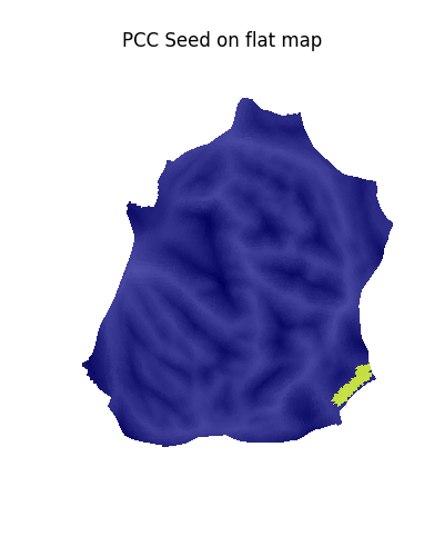
Using a flat mesh can be useful in order to easily locate the area of interest on the cortex. To make this plot easier to read, we use the mesh curvature as a background map.

bg_map = load_fsaverage_data(data_type="curvature")
for hemi, data in bg_map.data.parts.items():
    tmp = np.sign(data)
    # np.sign yields values in [-1, 1].
    # We rescale the background map
    # such that values are in [0.25, 0.75],
    # resulting in a nicer looking plot.
    tmp = (tmp + 1) / 4 + 0.25
    bg_map.data.parts[hemi]

plot_surf_roi(
    surf_mesh=fsaverage_meshes["flat"],
    roi_map=pcc_mask,
    hemi=hemisphere,
    view="dorsal",
    bg_map=fsaverage_sulcal,
    bg_on_data=True,
    title="PCC Seed on flat map",
)

show()

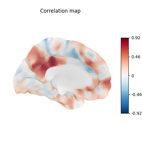
Calculating seed-based functional connectivity

Calculate Pearson product-moment correlation coefficient between seed time series and timeseries of all cortical nodes.

from scipy.stats import pearsonr

# Let's in initialize the data
# we will use to create our results image.
results = {}
for hemi, mesh in surf_img_nki.mesh.parts.items():
    n_vertices = mesh.n_vertices
    results[hemi] = np.zeros(n_vertices)

# Let's avoid computing results
# in unknown regions
# and on the medial wall.
excluded_labels = [
    destrieux.labels.index("Unknown"),
    destrieux.labels.index("Medial_wall"),
]
is_excluded = np.isin(
    destrieux_atlas.data.parts[hemisphere],
    excluded_labels,
)
for i, exclude_this_vertex in enumerate(is_excluded):
    if exclude_this_vertex:
        continue
    y = surf_img_nki.data.parts[hemisphere][i, ...]
    results[hemisphere][i] = pearsonr(seed_timeseries, y)[0]

stat_map_surf = SurfaceImage(
    mesh=destrieux_atlas.mesh,
    data=results,
)

Viewing results

Display unthresholded stat map with a slightly dimmed background

from nilearn.plotting import plot_surf_stat_map

plot_surf_stat_map(
    stat_map=stat_map_surf,
    hemi=hemisphere,
    view="medial",
    colorbar=True,
    bg_map=fsaverage_sulcal,
    bg_on_data=True,
    darkness=0.3,
    title="Correlation map",
)

show()

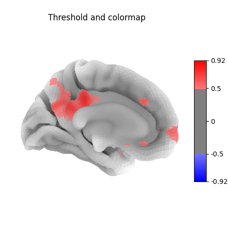
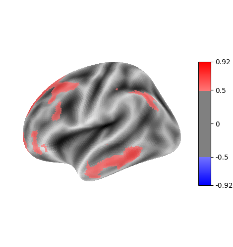
Many different options are available for plotting, for example thresholding, or using custom colormaps

plot_surf_stat_map(
    stat_map=stat_map_surf,
    hemi=hemisphere,
    view="medial",
    colorbar=True,
    bg_map=fsaverage_sulcal,
    bg_on_data=True,
    cmap="bwr",
    threshold=0.5,
    title="Threshold and colormap",
)

show()

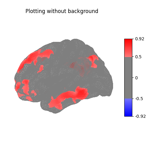
Here the surface is plotted in a lateral view without a background map. To capture 3D structure without depth information, the default is to plot a half transparent surface. Note that you can also control the transparency with a background map using the alpha parameter.

plot_surf_stat_map(
    stat_map=stat_map_surf,
    hemi=hemisphere,
    view="lateral",
    colorbar=True,
    cmap="bwr",
    threshold=0.5,
    title="Plotting without background",
)

show()

The plots can be saved to file, in which case the display is closed after creating the figure

from pathlib import Path

output_dir = Path.cwd() / "results" / "plot_surf_stat_map"
output_dir.mkdir(exist_ok=True, parents=True)
print(f"Output will be saved to: {output_dir}")

plot_surf_stat_map(
    surf_mesh=fsaverage_meshes["inflated"],
    stat_map=stat_map_surf,
    hemi=hemisphere,
    bg_map=fsaverage_sulcal,
    bg_on_data=True,
    threshold=0.5,
    colorbar=True,
    output_file=output_dir / "plot_surf_stat_map.png",
    cmap="bwr",
)

Output will be saved to: /home/runner/work/nilearn/nilearn/examples/01_plotting/results/plot_surf_stat_map

References

Estimated memory usage: 871 MB