Predicted time series and residuals

Here we fit a First Level GLM with the minimize_memory-argument set to False. By doing so, the FirstLevelModel-object stores the residuals, which we can then inspect. Also, the predicted time series can be extracted, which is useful to assess the quality of the model fit.

Warning

If you are using Nilearn with a version older than 0.9.0, then you should either upgrade your version or import maskers from the input_data module instead of the maskers module.

That is, you should manually replace in the following example all occurrences of:

from nilearn.maskers import NiftiMasker

with:

from nilearn.input_data import NiftiMasker

Import modules

import pandas as pd

from nilearn import image, masking
from nilearn.datasets import fetch_spm_auditory
from nilearn.plotting import plot_stat_map, show

# load fMRI data
subject_data = fetch_spm_auditory()
fmri_img = subject_data.func[0]

# Make an average
mean_img = image.mean_img(fmri_img)
mask = masking.compute_epi_mask(mean_img)

# Clean and smooth data
fmri_img = image.clean_img(fmri_img, standardize=None)
fmri_img = image.smooth_img(fmri_img, 5.0)

# load events
events = pd.read_csv(subject_data.events, sep="\t")

[fetch_spm_auditory] Dataset found in /home/runner/nilearn_data/spm_auditory

Fit model

Note that minimize_memory is set to False so that FirstLevelModel stores the residuals. signal_scaling is set to False, so we keep the same scaling as the original data in fmri_img.

from nilearn.glm.first_level import FirstLevelModel

fmri_glm = FirstLevelModel(
    t_r=subject_data.t_r,
    drift_model="cosine",
    signal_scaling=False,
    mask_img=mask,
    minimize_memory=False,
    verbose=1,
)

fmri_glm = fmri_glm.fit(fmri_img, events)

[FirstLevelModel.fit] Loading data from <nibabel.nifti1.Nifti1Image object at
0x7f9c478a4040>
[FirstLevelModel.fit] Loading mask from <nibabel.nifti1.Nifti1Image object at
0x7f9c478a7f70>
[FirstLevelModel.fit] Resampling mask
[FirstLevelModel.fit] Finished fit
[FirstLevelModel.fit] Computing run 1 out of 1 runs (go take a coffee, a big
one).
[FirstLevelModel.fit] Performing mask computation.
[FirstLevelModel.fit] Loading data from <nibabel.nifti1.Nifti1Image object at
0x7f9c478a4040>
[FirstLevelModel.fit] Extracting region signals
[FirstLevelModel.fit] Cleaning extracted signals
[FirstLevelModel.fit] Masking took 0 seconds.
[FirstLevelModel.fit] Performing GLM computation.
[FirstLevelModel.fit] GLM took 1 seconds.
[FirstLevelModel.fit] Computation of 1 runs done in 1 seconds.

Calculate and plot contrast

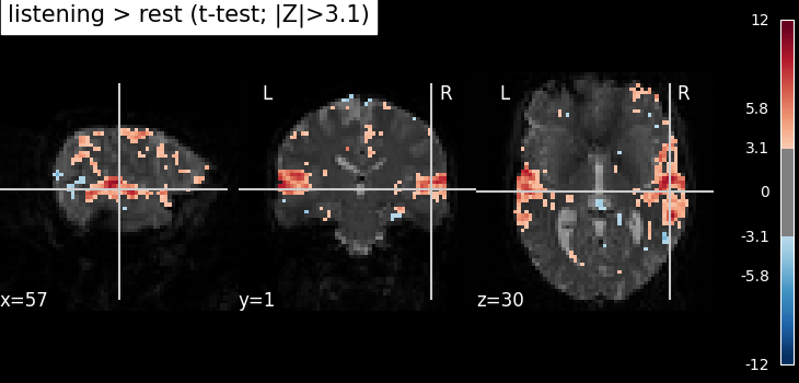
z_map = fmri_glm.compute_contrast("listening")

threshold = 3.1
plot_stat_map(
    z_map,
    bg_img=mean_img,
    threshold=threshold,
    title=f"listening > rest (t-test; |Z|>{threshold})",
)

show()

[FirstLevelModel.compute_contrast] Computing image from signals

Extract the largest clusters

We can extract the 6 largest clusters surviving our threshold. and get the x, y, and z coordinates of their peaks. We then extract the time series from a sphere around each coordinate.

from nilearn.maskers import NiftiSpheresMasker
from nilearn.reporting import get_clusters_table

table = get_clusters_table(
    z_map, stat_threshold=threshold, cluster_threshold=20
)
table.set_index("Cluster ID", drop=True)
print(table)

coords = table.loc[range(1, 7), ["X", "Y", "Z"]].to_numpy()
print(coords)

masker = NiftiSpheresMasker(coords, verbose=1)
real_timeseries = masker.fit_transform(fmri_img)
predicted_timeseries = masker.fit_transform(fmri_glm.predicted[0])

   Cluster ID     X     Y     Z  Peak Stat Cluster Size (mm3)
0           1 -60.0  -6.0  42.0  11.543910              20196
1          1a -51.0 -12.0  39.0  10.497958
2          1b -39.0 -12.0  39.0  10.118978
3          1c -63.0  12.0  33.0   9.754835
4           2  60.0   0.0  36.0  11.088600              32157
..        ...   ...   ...   ...        ...                ...
58         21  27.0 -72.0  27.0   4.422543                729
59        21a  24.0 -66.0  18.0   4.346647
60        21b  24.0 -78.0  21.0   3.428392
61         22 -30.0 -24.0  90.0   3.877083                648
62        22a -33.0 -18.0  72.0   3.791863

[63 rows x 6 columns]
[[-51. -12.  39.]
 [-39. -12.  39.]
 [-63.  12.  33.]
 [ 60.   0.  36.]
 [ 66.  12.  27.]
 [ 60. -18.  30.]]
[NiftiSpheresMasker.wrapped] Finished fit
[NiftiSpheresMasker.wrapped] Loading data from <nibabel.nifti1.Nifti1Image
object at 0x7f9c478a4040>
[NiftiSpheresMasker.wrapped] Extracting region signals
[NiftiSpheresMasker.wrapped] Cleaning extracted signals
[FirstLevelModel.predicted] Computing image from signals
[NiftiSpheresMasker.wrapped] Finished fit
[NiftiSpheresMasker.wrapped] Loading data from <nibabel.nifti1.Nifti1Image
object at 0x7f9c47c68820>
[NiftiSpheresMasker.wrapped] Extracting region signals
[NiftiSpheresMasker.wrapped] Cleaning extracted signals

Let’s have a look at the report to make sure the spheres are well placed.

report = masker.generate_report()
report

NiftiSpheresMasker Class for masking of Niimg-like objects using seeds. NiftiSpheresMasker is useful when data from given seeds should be extracted. Use case: summarize brain signals from seeds that were obtained from prior knowledge.

Previous Sphere

Next Sphere

This report shows the regions defined by the spheres of the masker.

The masker has 6 spheres in total (displayed together on the first image).

They can be individually browsed using Previous and Next buttons.

Regions summary

seed number	coordinates	position	radius	size (in mm^3)	size (in voxels)	relative size (in %)
0	[-51.0, -12.0, 39.0]	[48, 27, 35]	1.0	4.19	not implemented	not implemented
1	[-39.0, -12.0, 39.0]	[44, 27, 35]	1.0	4.19	not implemented	not implemented
2	[-63.0, 12.0, 33.0]	[52, 35, 33]	1.0	4.19	not implemented	not implemented
3	[60.0, 0.0, 36.0]	[11, 31, 34]	1.0	4.19	not implemented	not implemented
4	[66.0, 12.0, 27.0]	[9, 35, 31]	1.0	4.19	not implemented	not implemented
5	[60.0, -18.0, 30.0]	[11, 25, 32]	1.0	4.19	not implemented	not implemented

	Value
Parameter
allow_overlap	False
detrend	False
high_variance_confounds	False
memory_level	1
reports	True
seeds	[[-51.0, -12.0, 39.0], [-39.0, -12.0, 39.0], [-63.0, 12.0, 33.0], [60.0, 0.0, 36.0], [66.0, 12.0, 27.0], [60.0, -18.0, 30.0]]
standardize	False
standardize_confounds	True
verbose	1

Plot predicted and actual time series for 6 most significant clusters

import matplotlib.pyplot as plt

# colors for each of the clusters
colors = ["blue", "navy", "purple", "magenta", "olive", "teal"]
# plot the time series and corresponding locations
fig1, axs1 = plt.subplots(2, 6)
for i in range(6):
    # plotting time series
    axs1[0, i].set_title(f"Cluster peak {coords[i]}\n")
    axs1[0, i].plot(real_timeseries[:, i], c=colors[i], lw=2)
    axs1[0, i].plot(predicted_timeseries[:, i], c="r", ls="--", lw=2)
    axs1[0, i].set_xlabel("Time")
    axs1[0, i].set_ylabel("Signal intensity", labelpad=0)
    # plotting image below the time series
    roi_img = plot_stat_map(
        z_map,
        cut_coords=[coords[i][2]],
        threshold=3.1,
        figure=fig1,
        axes=axs1[1, i],
        display_mode="z",
        colorbar=False,
        bg_img=mean_img,
    )
    roi_img.add_markers([coords[i]], colors[i], 300)
fig1.set_size_inches(24, 14)

show()

Get residuals

resid = masker.fit_transform(fmri_glm.residuals[0])

[FirstLevelModel.residuals] Computing image from signals
[NiftiSpheresMasker.wrapped] Finished fit
[NiftiSpheresMasker.wrapped] Loading data from <nibabel.nifti1.Nifti1Image
object at 0x7f9c1d9c51b0>
[NiftiSpheresMasker.wrapped] Extracting region signals
[NiftiSpheresMasker.wrapped] Cleaning extracted signals

Plot distribution of residuals

Note that residuals are not really distributed normally.

fig2, axs2 = plt.subplots(2, 3, constrained_layout=True)

axs2 = axs2.flatten()
for i in range(6):
    axs2[i].set_title(f"Cluster peak {coords[i]}\n")
    axs2[i].hist(resid[:, i], color=colors[i])
    print(f"Mean residuals: {resid[:, i].mean()}")

fig2.set_size_inches(12, 7)

show()

Mean residuals: 0.018869405610299532
Mean residuals: 0.045756026122034346
Mean residuals: -1.5670004976137923e-14
Mean residuals: -0.13042393047259077
Mean residuals: -0.01499899481931678
Mean residuals: 0.049556260499625526

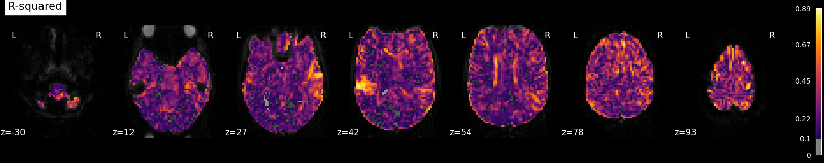
Plot R-squared

Because we stored the residuals, we can plot the R-squared: the proportion of explained variance of the GLM as a whole. Note that the R-squared is markedly lower deep down the brain, where there is more physiological noise and we are further away from the receive coils. However, R-Squared should be interpreted with a grain of salt. The R-squared value will necessarily increase with the addition of more factors (such as rest, active, drift, motion) into the GLM. Additionally, we are looking at the overall fit of the model, so we are unable to say whether a voxel/region has a large R-squared value because the voxel/region is responsive to the experiment (such as active or rest) or because the voxel/region fits the noise factors (such as drift or motion) that could be present in the GLM. To isolate the influence of the experiment, we can use an F-test as shown in the next section.

plot_stat_map(
    fmri_glm.r_square[0],
    bg_img=mean_img,
    threshold=0.1,
    display_mode="z",
    cut_coords=7,
    cmap="inferno",
    title="R-squared",
    vmin=0,
    symmetric_cbar=False,
)

[FirstLevelModel.r_square] Computing image from signals

<nilearn.plotting.displays._slicers.ZSlicer object at 0x7f9c2c9519c0>

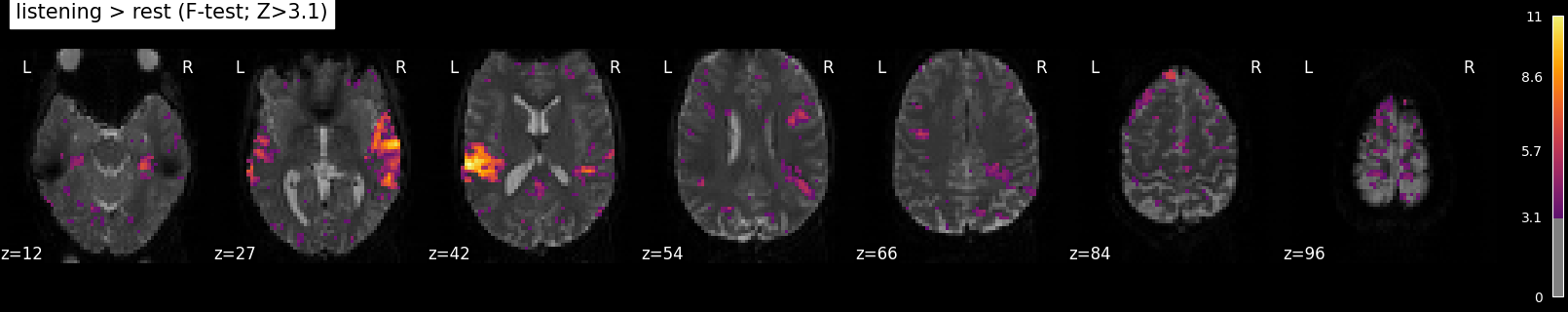
Calculate and Plot F-test

The F-test tells you how well the GLM fits effects of interest such as the active and rest conditions together. This is different from R-squared, which tells you how well the overall GLM fits the data, including active, rest and all the other columns in the design matrix such as drift and motion.

# f-test for 'listening'
z_map_ftest = fmri_glm.compute_contrast(
    "listening", stat_type="F", output_type="z_score"
)

plot_stat_map(
    z_map_ftest,
    bg_img=mean_img,
    threshold=threshold,
    display_mode="z",
    cut_coords=7,
    cmap="inferno",
    title=f"listening > rest (F-test; Z>{threshold})",
    symmetric_cbar=False,
    vmin=0,
)

show()

[FirstLevelModel.compute_contrast] Computing image from signals

Estimated memory usage: 772 MB