Decoding with FREM: face vs house vs chair object recognition

This example uses fast ensembling of regularized models (FREM) to decode a face vs house vs chair discrimination task from Haxby et al.[1] study. FREM uses an implicit spatial regularization through fast clustering and aggregates a high number of estimators trained on various splits of the training set, thus returning a very robust decoder at a lower computational cost than other spatially regularized methods.

To have more details, see: FREM: fast ensembling of regularized models for robust decoding.

Load the Haxby dataset

from nilearn.datasets import fetch_haxby

data_files = fetch_haxby()

[get_dataset_dir] Dataset found in /home/runner/nilearn_data/haxby2001

Load behavioral data

import pandas as pd

behavioral = pd.read_csv(data_files.session_target[0], sep=" ")

Restrict to face, house, and chair conditions

conditions = behavioral["labels"]
condition_mask = conditions.isin(["face", "house", "chair"])

Split data into train and test samples, using the chunks

condition_mask_train = (condition_mask) & (behavioral["chunks"] <= 6)
condition_mask_test = (condition_mask) & (behavioral["chunks"] > 6)

Apply this sample mask to X (fMRI data) and y (behavioral labels) Because the data is in one single large 4D image, we need to use index_img to do the split easily

from nilearn.image import index_img

func_filenames = data_files.func[0]
X_train = index_img(func_filenames, condition_mask_train)
X_test = index_img(func_filenames, condition_mask_test)
y_train = conditions[condition_mask_train].to_numpy()
y_test = conditions[condition_mask_test].to_numpy()

Compute the mean EPI to be used for the background of the plotting

from nilearn.image import mean_img

background_img = mean_img(func_filenames, copy_header=True)

Fit FREM

from nilearn.decoding import FREMClassifier

Restrict analysis to within the brain mask

mask = data_files.mask

decoder = FREMClassifier(
    mask=mask, cv=10, standardize="zscore_sample", n_jobs=2, verbose=1
)

Fit model on train data and predict on test data

decoder.fit(X_train, y_train)
y_pred = decoder.predict(X_test)
accuracy = (y_pred == y_test).mean() * 100.0
print(f"FREM classification accuracy : {accuracy:g}%")

[FREMClassifier.fit] Loading data from None
[FREMClassifier.fit] Resampling mask
[FREMClassifier.fit] Finished fit
[FREMClassifier.fit] Loading data from Nifti1Image(
shape=(40, 64, 64, 189),
affine=array([[  -3.5  ,    0.   ,    0.   ,   68.25 ],
       [   0.   ,    3.75 ,    0.   , -118.125],
       [   0.   ,    0.   ,    3.75 , -118.125],
       [   0.   ,    0.   ,    0.   ,    1.   ]])
)
[FREMClassifier.fit] Extracting region signals
[FREMClassifier.fit] Cleaning extracted signals
[Parallel(n_jobs=2)]: Using backend LokyBackend with 2 concurrent workers.
[Parallel(n_jobs=2)]: Done  30 out of  30 | elapsed:   21.8s finished
[FREMClassifier.predict] Loading data from Nifti1Image(
shape=(40, 64, 64, 135),
affine=array([[  -3.5  ,    0.   ,    0.   ,   68.25 ],
       [   0.   ,    3.75 ,    0.   , -118.125],
       [   0.   ,    0.   ,    3.75 , -118.125],
       [   0.   ,    0.   ,    0.   ,    1.   ]])
)
[FREMClassifier.predict] Extracting region signals
[FREMClassifier.predict] Cleaning extracted signals
FREM classification accuracy : 60.7407%

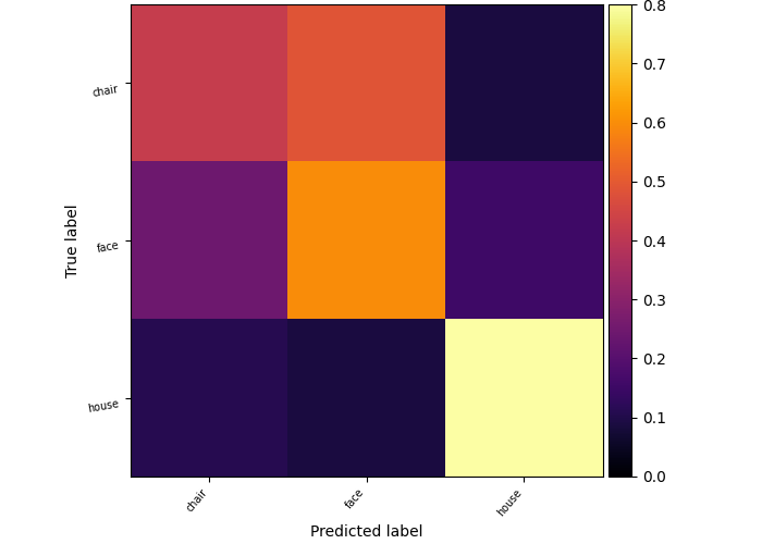
Plot confusion matrix

import numpy as np
from sklearn.metrics import confusion_matrix

from nilearn.plotting import plot_matrix, plot_stat_map, show

Calculate the confusion matrix

matrix = confusion_matrix(
    y_test,
    y_pred,
    normalize="true",
)

Plot the confusion matrix

im = plot_matrix(
    matrix,
    labels=sorted(np.unique(y_test)),
    vmin=0,
    cmap="inferno",
)

# Add x/y-axis labels
ax = im.axes
ax.set_ylabel("True label")
ax.set_xlabel("Predicted label")

show()

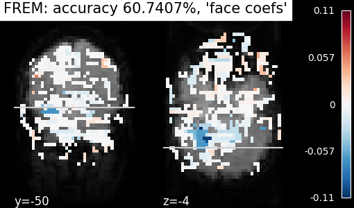
Visualization of FREM weights

plot_stat_map(
    decoder.coef_img_["face"],
    background_img,
    title=f"FREM: accuracy {accuracy:g}%, 'face coefs'",
    cut_coords=(-50, -4),
    display_mode="yz",
)
show()

FREM ensembling procedure yields an important improvement of decoding accuracy on this simple example compared to fitting only one model per fold and the clustering mechanism keeps its computational cost reasonable even on heavier examples. Here we ensembled several instances of l2-SVC, but FREMClassifier also works with ridge or logistic. FREMRegressor object is also available to solve regression problems.

References

[1]

James V. Haxby, M. Ida Gobbini, Maura L. Furey, Alumit Ishai, Jennifer L. Schouten, and Pietro Pietrini. Distributed and overlapping representations of faces and objects in ventral temporal cortex. Science, 293(5539):2425–2430, 2001. doi:10.1126/science.1063736.

Estimated memory usage: 1014 MB