A short demo of the surface images & maskers

This example shows some more ‘advanced’ features to work with surface images.

This shows:

• how to use SurfaceMasker and to plot SurfaceImage

• how to use SurfaceLabelsMasker and to compute a connectome with surface data.

• how to use run some decoding directly on surface data.

from nilearn._utils.helpers import check_matplotlib

check_matplotlib()

Masking and plotting surface images

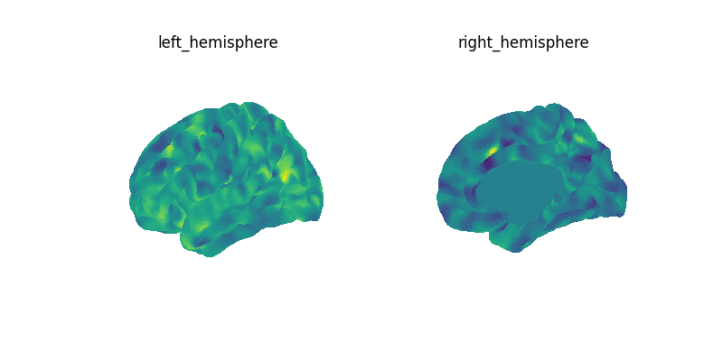
Here we load the NKI dataset as a list of SurfaceImage. Then we extract data with a masker and compute the mean image across time points for the first subject. We then plot the the mean image.

import matplotlib.pyplot as plt
import numpy as np

from nilearn.datasets import (
    load_fsaverage_data,
    load_nki,
)
from nilearn.maskers import SurfaceMasker
from nilearn.plotting import plot_matrix, plot_surf, show

surf_img_nki = load_nki()[0]
print(f"NKI image: {surf_img_nki}")

masker = SurfaceMasker()
masked_data = masker.fit_transform(surf_img_nki)
print(f"Masked data shape: {masked_data.shape}")

mean_data = masked_data.mean(axis=0)
mean_img = masker.inverse_transform(mean_data)
print(f"Image mean: {mean_img}")

# let's create a figure with all the views for both hemispheres
views = [
    "lateral",
    "medial",
    "dorsal",
    "ventral",
    "anterior",
    "posterior",
]
hemispheres = [
    "left",
    "right",
]

# for our plots we will be using the fsaverage sulcal data as background map
fsaverage_sulcal = load_fsaverage_data(data_type="sulcal")

fig, axes = plt.subplots(
    nrows=len(views),
    ncols=len(hemispheres),
    subplot_kw={"projection": "3d"},
    figsize=(4 * len(hemispheres), 4),
)
axes = np.atleast_2d(axes)

# Let's ensure that we have the same range
# centered on 0 for all subplots.
vmax = max(np.absolute(hemi).max() for hemi in mean_img.data.parts.values())
vmin = -vmax

for view, ax_row in zip(views, axes):
    for ax, hemi in zip(ax_row, hemispheres):
        plot_surf(
            surf_map=mean_img,
            hemi=hemi,
            view=view,
            figure=fig,
            axes=ax,
            title=f"mean image - {hemi} - {view}",
            colorbar=False,
            cmap="bwr",
            symmetric_cmap=True,
            bg_on_data=True,
            vmin=vmin,
            vmax=vmax,
            bg_map=fsaverage_sulcal,
        )
fig.set_size_inches(6, 8)

show()

[get_dataset_dir] Dataset found in
/home/runner/nilearn_data/nki_enhanced_surface
[load_nki] Loading subject 1 of 1.
NKI image: <SurfaceImage (20484, 895)>
Masked data shape: (895, 20484)
Image mean: <SurfaceImage (20484, 1)>

Connectivity with a surface atlas and SurfaceLabelsMasker

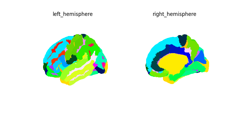
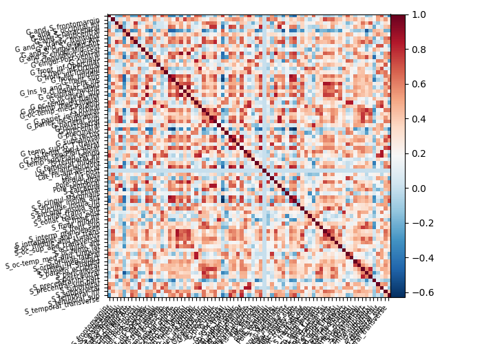
Here we first get the mean time serie for each label of the destrieux atlas for our NKI data. We then compute and plot the connectome of these time series.

from nilearn.connectome import ConnectivityMeasure
from nilearn.datasets import (
    fetch_atlas_surf_destrieux,
    load_fsaverage,
)
from nilearn.maskers import SurfaceLabelsMasker
from nilearn.surface import SurfaceImage

fsaverage = load_fsaverage("fsaverage5")
destrieux = fetch_atlas_surf_destrieux()

# Let's create a surface image
# for this atlas.
labels_img = SurfaceImage(
    mesh=fsaverage["pial"],
    data={
        "left": destrieux["map_left"],
        "right": destrieux["map_right"],
    },
)

# The labels are stored as bytes for the Destrieux atlas.
# For convenience we decode them to string.
label_names = [x.decode("utf-8") for x in destrieux.labels]

labels_masker = SurfaceLabelsMasker(
    labels_img=labels_img,
    labels=label_names,
).fit()

masked_data = labels_masker.transform(surf_img_nki)
print(f"Masked data shape: {masked_data.shape}")

[get_dataset_dir] Dataset found in /home/runner/nilearn_data/destrieux_surface
Masked data shape: (895, 75)

connectome_measure = ConnectivityMeasure(kind="correlation")
connectome = connectome_measure.fit([masked_data])
vmax = np.absolute(connectome.mean_).max()
vmin = -vmax
plot_matrix(
    connectome.mean_,
    labels=labels_masker.label_names_,
    vmax=vmax,
    vmin=vmin,
)

show()

Using the Decoder

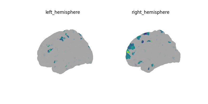
Now using the appropriate masker we can use a Decoder on surface data just as we do for volume images.

Note

Here we are given dummy 0 or 1 labels to each time point of the time series. We then decode at each time point. In this sense, the results do not show anything meaningful in a biological sense.

from nilearn.decoding import Decoder

# create some random labels
rng = np.random.RandomState(0)
n_time_points = surf_img_nki.shape[1]
y = rng.choice(
    [0, 1],
    replace=True,
    size=n_time_points,
)

decoder = Decoder(
    mask=SurfaceMasker(),
    param_grid={"C": [0.01, 0.1]},
    cv=3,
    screening_percentile=1,
)
decoder.fit(surf_img_nki, y)
print("CV scores:", decoder.cv_scores_)

plot_surf(
    surf_map=decoder.coef_img_[0],
    threshold=1e-6,
    bg_map=fsaverage_sulcal,
    bg_on_data=True,
    colorbar=True,
    cmap="black_red",
    vmin=0,
)
show()

/home/runner/work/nilearn/nilearn/.tox/doc/lib/python3.9/site-packages/nilearn/decoding/decoder.py:732: UserWarning:

Overriding provided-default estimator parameters with provided masker parameters :
Parameter standardize :
    Masker parameter False - overriding estimator parameter True


/home/runner/work/nilearn/nilearn/.tox/doc/lib/python3.9/site-packages/sklearn/feature_selection/_univariate_selection.py:112: UserWarning:

Features [    8    36    38 ... 20206 20207 20208] are constant.

/home/runner/work/nilearn/nilearn/.tox/doc/lib/python3.9/site-packages/sklearn/feature_selection/_univariate_selection.py:113: RuntimeWarning:

invalid value encountered in true_divide

/home/runner/work/nilearn/nilearn/.tox/doc/lib/python3.9/site-packages/sklearn/feature_selection/_univariate_selection.py:112: UserWarning:

Features [    8    36    38 ... 20206 20207 20208] are constant.

/home/runner/work/nilearn/nilearn/.tox/doc/lib/python3.9/site-packages/sklearn/feature_selection/_univariate_selection.py:113: RuntimeWarning:

invalid value encountered in true_divide

/home/runner/work/nilearn/nilearn/.tox/doc/lib/python3.9/site-packages/sklearn/feature_selection/_univariate_selection.py:112: UserWarning:

Features [    8    36    38 ... 20206 20207 20208] are constant.

/home/runner/work/nilearn/nilearn/.tox/doc/lib/python3.9/site-packages/sklearn/feature_selection/_univariate_selection.py:113: RuntimeWarning:

invalid value encountered in true_divide

CV scores: {0: [0.4991939095387371, 0.5115891053391053, 0.48466810966810964], 1: [0.4991939095387371, 0.5115891053391053, 0.48466810966810964]}

Decoding with a scikit-learn Pipeline

from sklearn import feature_selection, linear_model, pipeline, preprocessing

decoder = pipeline.make_pipeline(
    SurfaceMasker(),
    preprocessing.StandardScaler(),
    feature_selection.SelectKBest(
        score_func=feature_selection.f_regression, k=500
    ),
    linear_model.Ridge(),
)
decoder.fit(surf_img_nki, y)

coef_img = decoder[:-1].inverse_transform(np.atleast_2d(decoder[-1].coef_))

vmax = max(np.absolute(hemi).max() for hemi in coef_img.data.parts.values())
vmin = -vmax
plot_surf(
    surf_map=coef_img,
    cmap="bwr",
    vmin=vmin,
    vmax=vmax,
    threshold=1e-6,
    bg_map=fsaverage_sulcal,
    bg_on_data=True,
    colorbar=True,
)
show()

Estimated memory usage: 1349 MB