Understanding Decoder

Nilearn’s Decoder object is a composite estimator that does several things under the hood and can hence be a bit difficult to understand at first.

This example aims to provide a clear understanding of the Decoder object by demonstrating these steps via a Scikit-Learn pipeline.

We will use the Haxby et al.[1] dataset where the participants were shown images of 8 different types as described in the Decoding with ANOVA + SVM: face vs house in the Haxby dataset example. We will train a classifier to predict the label of the object in the stimulus image based on the subject’s fMRI data from the Ventral Temporal cortex.

Load the Haxby dataset

from nilearn import datasets

# By default 2nd subject data will be fetched on which we run our analysis
haxby_dataset = datasets.fetch_haxby()
fmri_img = haxby_dataset.func[0]
# Pick the mask that we will use to extract the data from Ventral Temporal
# cortex
mask_vt = haxby_dataset.mask_vt[0]

# Load the behavioral data
import pandas as pd

from nilearn.image import index_img

behavioral_data = pd.read_csv(haxby_dataset.session_target[0], sep=" ")
labels = behavioral_data["labels"]
# Keep the trials corresponding to all the labels except the ``rest`` ones
labels_mask = labels != "rest"
y = labels[labels_mask]
y = y.to_numpy()

# Load run information
run = behavioral_data["chunks"][labels_mask]
run = run.to_numpy()

# Also keep the fmri data corresponding to these labels
fmri_img = index_img(fmri_img, labels_mask)

# Overview of the input data
import numpy as np

n_labels = len(np.unique(y))

print(f"{n_labels} labels to predict (y): {np.unique(y)}")
print(f"fMRI data shape (X): {fmri_img.shape}")
print(f"Runs (groups): {np.unique(run)}")

[fetch_haxby] Dataset found in /home/runner/nilearn_data/haxby2001
8 labels to predict (y): ['bottle' 'cat' 'chair' 'face' 'house' 'scissors' 'scrambledpix' 'shoe']
fMRI data shape (X): (40, 64, 64, 864)
Runs (groups): [ 0  1  2  3  4  5  6  7  8  9 10 11]

Preprocessing

As we can see, the fMRI data is a 4D image with shape (40, 64, 64, 864). Here 40x64x64 are the dimensions of the 3D brain image and 864 is the number of brain volumes acquired while visual stimuli were presented, each corresponding to one of the 8 labels we selected above.

Decoder can convert this 4D image to a 2D numpy array where each row corresponds to a trial and each column corresponds to a voxel. In addition, it can also do several other things like masking, smoothing, standardizing the data etc. depending on your requirements.

Under the hood, Decoder uses NiftiMasker to do all these operations. So here we will demonstrate this by directly using the NiftiMasker. Specifically, we will use it to:

1. only keep the data from the Ventral Temporal cortex by providing the mask image (in Decoder this is done by providing the mask image in the mask parameter).

2. standardize the data by z-scoring it such that the data is scaled to have zero mean and unit variance across trials (in Decoder this is done by setting the standardize parameter to "zscore_sample").

from nilearn.maskers import NiftiMasker

masker = NiftiMasker(mask_img=mask_vt, standardize="zscore_sample")

Convert the multi-class labels to binary labels

The Decoder converts multi-class classification problem to N one-vs-others binary classification problems by default (where N is the number of unique labels)

The advantage of this approach is its interpretability. Once we are done with training and cross-validating, we will have N area-under receiver operating characteristic curve (AU-ROC) scores, one for each label. This will give us an insight into which labels (and the corresponding cognitive domains) are easier to predict and are hence well differentiated relative to the others in the brain.

In addition, we will also have access to the classifier coefficients for each label. These can be further used to understand the importance of each voxel for each corresponding cognitive domain.

In this example we have N = 8 unique labels and we will use Scikit-Learn’s LabelBinarizer to do this conversion.

from matplotlib import pyplot as plt
from sklearn.preprocessing import LabelBinarizer

label_binarizer = LabelBinarizer(pos_label=1, neg_label=-1)
y_binary = label_binarizer.fit_transform(y)

Let’s plot the labels to understand the conversion

from matplotlib.colors import ListedColormap
from sklearn.preprocessing import LabelEncoder

# create a copy of y_binary and manipulate it just for plotting
y_binary_ = y_binary.copy()
for col in range(y_binary_.shape[1]):
    y_binary_[np.where(y_binary_[:, col] == 1), col] = col

fig, (ax_binary, ax_multi) = plt.subplots(
    2, gridspec_kw={"height_ratios": [10, 1.5]}, figsize=(12, 2)
)
cmap = ListedColormap(["white", *list(plt.cm.tab10.colors)[:n_labels]])
binary_plt = ax_binary.imshow(
    y_binary_.T,
    aspect="auto",
    cmap=cmap,
    interpolation="nearest",
    origin="lower",
)
ax_binary.set_xticks([])
ax_binary.set_yticks([])
ax_binary.set_ylabel("One-vs-Others")

# encode the original labels for plotting
label_multi = LabelEncoder()
y_multi = label_multi.fit_transform(y)
y_multi = y_multi.reshape(1, -1)
cmap = ListedColormap(list(plt.cm.tab10.colors)[:n_labels])
multi_plt = ax_multi.imshow(
    y_multi,
    aspect="auto",
    interpolation="nearest",
    cmap=cmap,
)
ax_multi.set_yticks([])
ax_multi.set_xlabel("Original trial sequence")
cbar = fig.colorbar(multi_plt, ax=[ax_binary, ax_multi])
cbar.set_ticks(np.arange(1 + len(label_multi.classes_)))
cbar.set_ticklabels([*label_multi.classes_, "all others"])

plt.show()

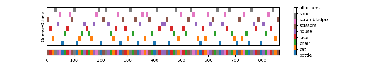
So at the bottom we have the original presentation sequence of the selected trials and at the top we have the labels in the one-vs-others format.

Each row corresponds to a one-vs-others binary classification problem. For example, the first row from the bottom corresponds to the binary classification problem of predicting the label “bottle” vs. all other labels and so on. Later we will train a classifier for each row and calculate the AU-ROC score for each row.

Feature selection

After preprocessing the provided fMRI data, the Decoder performs a univariate feature selection on the voxels of the brain volume. It uses Scikit-Learn’s SelectPercentile with f_classif to calculate ANOVA F-scores for each voxel and to only keep the ones that have highest 20 percentile scores, by default. This selection threshold can be changed using the screening_percentile parameter.

These 20 percentile voxels are with respect to the volume of the standard MNI152 brain template. Furthermore, if the provided mask image has less voxels than the selected percentile, all voxels in the mask are used.

Also note that these top 20 percentile voxels are selected based on training set and then these selected voxels are picked for the test set too for each train-test split.

For simplicity we will just keep all (100 percentile) voxels in this example.

from sklearn.feature_selection import SelectPercentile, f_classif

screening_percentile = 100
feature_selector = SelectPercentile(f_classif, percentile=screening_percentile)

Hyperparameter optimization

The Decoder also performs hyperparameter tuning. How this is done depends on the estimator used.

For the support vector classifiers (known as SVC, and used by setting estimator="svc" or "svc_l1" or "svc_l2"), the score from the best performing regularization hyperparameter (C) for each train-test split is picked.

For all classifiers other than SVC, the hyperparameter tuning is done using the <estimator_name>CV classes from Scikit-Learn. This essentially means that the hyperparameters are optimized using an internal cross-validation on the training data.

In addition, the parameter grids that are used for hyperparameter tuning by Decoder are also different from the default Scikit-Learn parameter grids for the corresponding <estimator_name>CV objects.

For simplicity, let’s use Scikit-Learn’s LogisticRegressionCV with custom parameter grid (via Cs parameter) as used in Nilearn’s Decoder.

from sklearn.linear_model import LogisticRegressionCV

classifier = LogisticRegressionCV(
    penalty="l2",
    solver="liblinear",
    Cs=np.geomspace(1e-3, 1e4, 8),
    refit=True,
)

Leave out a test set for final evaluation

Before we train and cross-validate, let’s leave out one run as a final test set to evaluate the performance of the trained decoder on unseen data.

test_run = 6
test_mask = run == test_run

# training data for cross-validation
fmri_img_cv = index_img(fmri_img, ~test_mask)
y_cv = y[~test_mask]
y_binary_cv = y_binary[~test_mask]
run_cv = run[~test_mask]

# Transform fMRI data into a 2D numpy array and standardize it with the masker
X_cv = masker.fit_transform(fmri_img_cv)

# test data
fmri_img_test = index_img(fmri_img, test_mask)
X_test = masker.transform(fmri_img_test)
y_test = y_binary[test_mask]
run_test = run[test_mask]

/home/runner/work/nilearn/nilearn/examples/02_decoding/plot_haxby_understand_decoder.py:254: UserWarning: [NiftiMasker.fit] Generation of a mask has been requested (imgs != None) while a mask was given at masker creation. Given mask will be used.
  X_cv = masker.fit_transform(fmri_img_cv)

Train and cross-validate via an Scikit-Learn pipeline

Now let’s put all the pieces together to train and cross-validate. The Decoder uses a leave-one-group-out cross-validation scheme by default in cases where groups are defined. In our example a group is a run, so we will use Scikit-Learn’s LeaveOneGroupOut

from sklearn.metrics import roc_auc_score
from sklearn.model_selection import LeaveOneGroupOut

logo_cv = LeaveOneGroupOut()

print(f"fMRI data shape after masking: {X_cv.shape}")
# So now we have a 2D numpy array where each row corresponds to a trial and
# each column corresponds to a feature (voxel in the Ventral Temporal cortex).

# Loop over each CV split and each class vs. rest binary classification
# problems (number of classification problems = n_labels)
scores_sklearn = []
coefs_sklearn = []
intercepts_sklearn = []
for klass in range(n_labels):
    for train, val in logo_cv.split(X_cv, groups=run_cv):
        # separate train and val events in the data
        X_train, X_val = X_cv[train], X_cv[val]
        # separate labels for train and val events for a given class vs. rest
        # problem
        y_train, y_val = (
            y_binary_cv[train, klass],
            y_binary_cv[val, klass],
        )

        # select the voxels by fitting feature selector on training data
        X_train = feature_selector.fit_transform(X_train, y_train)
        # pick the same voxels in the val data
        X_val = feature_selector.transform(X_val)

        # fit the classifier on the training data
        classifier.fit(X_train, y_train)
        # predict the labels on the val data
        pred = classifier.predict_proba(X_val)

        # calculate the ROC AUC score
        score = roc_auc_score(y_val, pred[:, 1])
        scores_sklearn.append(score)

        coefs_sklearn.append(classifier.coef_)
        intercepts_sklearn.append(classifier.intercept_)

fMRI data shape after masking: (792, 464)

Decode via the Decoder

All these steps can be done in a few lines and made faster via parallel processing using the n_jobs parameter in Decoder.

from nilearn.decoding import Decoder

decoder = Decoder(
    estimator="logistic_l2",
    mask=mask_vt,
    n_jobs=n_labels,
    cv=logo_cv,
    screening_percentile=screening_percentile,
    scoring="roc_auc_ovr",
)
decoder.fit(fmri_img_cv, y_cv, groups=run_cv)
scores_nilearn = np.concatenate(list(decoder.cv_scores_.values()))

/home/runner/work/nilearn/nilearn/examples/02_decoding/plot_haxby_understand_decoder.py:331: UserWarning: [NiftiMasker.fit] Generation of a mask has been requested (imgs != None) while a mask was given at masker creation. Given mask will be used.
  decoder.fit(fmri_img_cv, y_cv, groups=run_cv)

Compare the results

Let’s compare the results from the Scikit-Learn pipeline and the Nilearn decoder.

print("Nilearn mean AU-ROC score", np.mean(scores_nilearn))
print("Scikit-Learn mean AU-ROC score", np.mean(scores_sklearn))

Nilearn mean AU-ROC score 0.8988696488696489
Scikit-Learn mean AU-ROC score 0.8988295654962322

As we can see, the mean AU-ROC scores from the Scikit-Learn pipeline and Nilearn’s Decoder are identical.

The advantage of using Nilearn’s Decoder is that it does all these steps under the hood and provides a simple interface to train, cross-validate and predict on new data, while also parallelizing the computations to make the cross-validation faster. It also organizes the results in a structured way that can be easily accessed and analyzed.

Compare the coefficients and intercepts

The decoder object also provides access to the coefficients and intercepts of the trained classifiers for each class vs. rest problem. These are stored in the coef_ and intercept_ attributes of the decoder object, respectively. These coefficients and intercepts are averaged across the CV splits for each class vs. rest problem.

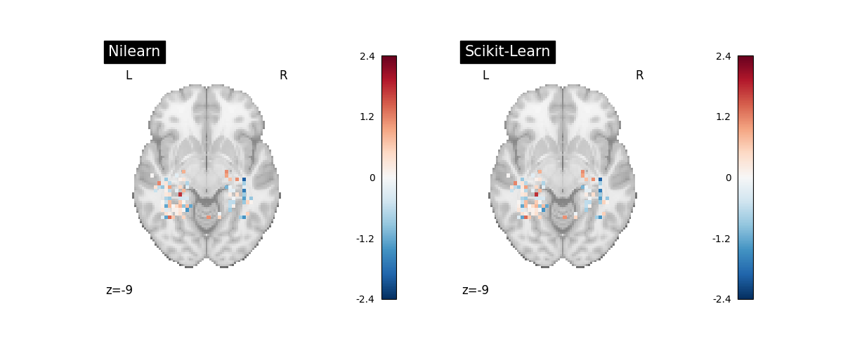
So we can aggregate the coefficients and intercepts from the Scikit-Learn pipeline by taking their mean across CV splits for each class vs. rest problem to check if they are comparable to the coefficients and intercepts from the Nilearn decoder.

from nilearn.plotting import plot_img_comparison, plot_stat_map, show

increment = len(np.unique(run_cv))

av_sklearn_coef = np.vstack(
    [
        np.mean(coefs_sklearn[i : i + increment], axis=0)
        for i in range(0, len(coefs_sklearn), increment)
    ]
)
av_sklearn_intercept = np.squeeze(
    np.vstack(
        [
            np.mean(intercepts_sklearn[i : i + increment], axis=0)
            for i in range(0, len(intercepts_sklearn), increment)
        ]
    )
)

fig, (ax_nilearn, ax_sklearn) = plt.subplots(1, 2, figsize=(12, 5))
plot_stat_map(
    decoder.coef_img_["bottle"],
    axes=ax_nilearn,
    display_mode="z",
    cut_coords=[-9],
    title="Nilearn",
)

plot_stat_map(
    masker.inverse_transform(av_sklearn_coef[0]),
    axes=ax_sklearn,
    display_mode="z",
    cut_coords=[-9],
    title="Scikit-Learn",
)
show()

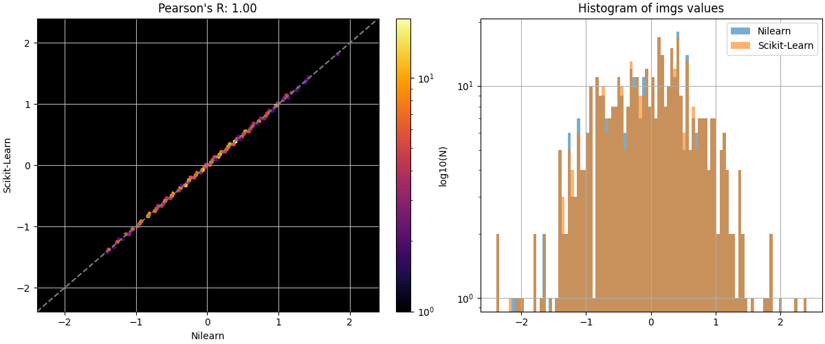
plot_img_comparison(
    decoder.coef_img_["bottle"],
    masker.inverse_transform(av_sklearn_coef[0]),
    decoder.masker_,
    ref_label="Nilearn",
    src_label="Scikit-Learn",
)
show()

• 
• 

/home/runner/work/nilearn/nilearn/examples/02_decoding/plot_haxby_understand_decoder.py:406: UserWarning: Standardization of 3D signal has been requested but would lead to zero values. Skipping.
  plot_img_comparison(

Note

The coefficients and intercepts from the Scikit-Learn pipeline and the Nilearn decoder are not identical. We’re unsure about the exact reason for this but the differences seem to depend on OS – they are bigger on Linux than on Mac. However they are not big enough to cause a difference in the predicted labels on the test set.

Compare the predicted labels on the left-out test set

Finally, the decoder object also uses these aggregated coefficients and intercepts to predict the labels on new data via its predict method. So if we also compare the predicted labels from the decoder and the Scikit-Learn pipeline on the left-out test set, we should see that they are also identical.

from sklearn.utils.extmath import safe_sparse_dot

# select the same voxels in the test data as selected in the training data
X_test = feature_selector.transform(X_test)

pred_nilearn = decoder.predict(X_test)
decision_function_sklearn = (
    safe_sparse_dot(X_test, av_sklearn_coef.T, dense_output=True)
    + av_sklearn_intercept
)
indices = decision_function_sklearn.argmax(axis=1)
pred_sklearn = decoder.classes_[indices]


print(
    "Predicted labels are identical:",
    (pred_nilearn == pred_sklearn).all(),
)

Predicted labels are identical: True

Estimated memory usage: 1413 MB