Note
This page is a reference documentation. It only explains the function signature, and not how to use it. Please refer to the user guide for the big picture.
nilearn.plotting.plot_roi
- nilearn.plotting.plot_roi(roi_img, bg_img=<MNI152Template>, cut_coords=None, output_file=None, display_mode='ortho', figure=None, axes=None, title=None, annotate=True, draw_cross=True, black_bg='auto', threshold=0.5, alpha=0.7, cmap='gist_ncar', dim='auto', colorbar=True, cbar_tick_format='%.2g', vmin=None, vmax=None, resampling_interpolation='nearest', view_type='continuous', linewidths=2.5, radiological=False, **kwargs)[source]
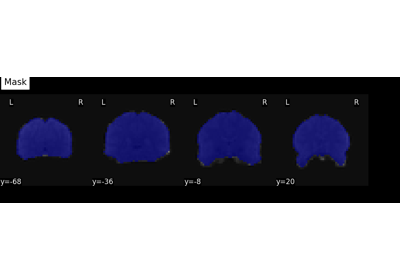
Plot cuts of an ROI/mask image.
By default 3 cuts: Frontal, Axial, and Lateral.
- Parameters:
- roi_imgNiimg-like object
See Input and output: neuroimaging data representation. The ROI/mask image, it could be binary mask or an atlas or ROIs with integer values.
- bg_imgNiimg-like object, optional
See Input and output: neuroimaging data representation. The background image to plot on top of. If nothing is specified, the MNI152 template will be used. To turn off background image, just pass “bg_img=None”. default=MNI152TEMPLATE.
- cut_coordsNone, allowed types depend on the
display_mode, optional The world coordinates of the point where the cut is performed.
If
display_modeis'ortho'or'tiled', this must be a 3-sequence offloatorint:(x, y, z).If
display_modeis'xz','yz'or'yx', this must be a 2-sequence offloatorint:(x, z),(y, z)or(x, y).If
display_modeis"x","y", or"z", this can be:If
display_modeis'mosaic', this can be:an
intin which case it specifies the number of cuts to perform in each direction"x","y","z".a 3-sequence of
floatorintin which case it specifies the number of cuts to perform in each direction"x","y","z"separately.dict<str: 1Dndarray> in which case keys are the directions (‘x’, ‘y’, ‘z’) and the values are sequences holding the cut coordinates.
If
Noneis given, the cuts are calculated automatically.
- output_file
strorpathlib.Pathor None, default=None The name of an image file to export the plot to. Valid extensions are .png, .pdf, .svg. If output_file is not None, the plot is saved to a file, and the display is closed.
- display_mode{“ortho”, “tiled”, “mosaic”, “x”, “y”, “z”, “yx”, “xz”, “yz”}, default=”ortho”
Choose the direction of the cuts:
"x": sagittal"y": coronal"z": axial"ortho": three cuts are performed in orthogonal directions"tiled": three cuts are performed and arranged in a 2x2 grid"mosaic": three cuts are performed along multiple rows and columns
- figure
int, ormatplotlib.figure.Figure, or None, optional Matplotlib figure used or its number. If None is given, a new figure is created.
- axes
matplotlib.axes.Axes, or 4tupleoffloat: (xmin, ymin, width, height), default=None The axes, or the coordinates, in matplotlib figure space, of the axes used to display the plot. If None, the complete figure is used.
- title
str, or None, default=None The title displayed on the figure.
- annotate
bool, default=True If annotate is True (like positions and / or left/right annotation) are added to the plot.
- draw_cross
bool, default=True If draw_cross is True, a cross is drawn on the plot to indicate the cut position.
- black_bg
bool, or “auto”, optional If True, the background of the image is set to be black. If you wish to save figures with a black background, you will need to pass facecolor=”k”, edgecolor=”k” to
matplotlib.pyplot.savefig. default=’auto’.- threshold
intorfloat,str, None, or ‘auto’, optional If None is given, the image is not thresholded. If number is given, it must be non-negative. The specified value is used to threshold the image: values below the threshold (in absolute value) are plotted as transparent. If a string percentile is given, it should finish with percent sign e.g., “95%”. We threshold based on the score obtained using this percentile on the image data. If “auto” is given, the threshold is determined based on the score obtained using percentile value “80%” on the absolute value of the image data. default=0.5.
- alpha
floatbetween 0 and 1, default=0.7 Alpha sets the transparency of the color inside the filled contours.
- cmap
matplotlib.colors.Colormap, orstr, orpandas.DataFrame, optional The colormap to use. Either a string which is a name of a matplotlib colormap, or a matplotlib colormap object, or a BIDS compliant look-up table passed as a pandas dataframe or a path to a tsv or csv file. If the look up table does not contain a
colorcolumn, then the default colormap of this function will be used.Warning
If the
namecolumn in the look up table does not contain abackgroundorBackgroundvalue, then the colormap will be shifted by one.See issue 5934.
default=`gist_ncar`.
- dim
float, or “auto”, optional Dimming factor applied to background image. By default, automatic heuristics are applied based upon the background image intensity. Accepted float values, where a typical span is between -2 and 2 (-2 = increase contrast; 2 = decrease contrast), but larger values can be used for a more pronounced effect. 0 means no dimming. default=’auto’.
- colorbar
bool, optional If True, display a colorbar next to the plots. default=True
- cbar_tick_format
str, default=”%i” Controls how to format the tick labels of the colorbar. Ex: use “%.2g” to use scientific notation.
- vmin
floator obj:int or None, optional Lower bound of the colormap. The values below vmin are masked. If None, the min of the image is used. Passed to
matplotlib.pyplot.imshow.- vmax
floator obj:int or None, optional Upper bound of the colormap. The values above vmax are masked. If None, the max of the image is used. Passed to
matplotlib.pyplot.imshow.- resampling_interpolation
str, optional Interpolation to use when resampling the image to the destination space. Can be:
"continuous": use 3rd-order spline interpolation"nearest": use nearest-neighbor mapping.
Note
"nearest"is faster but can be noisier in some cases.default=’nearest’.
- view_type{‘continuous’, ‘contours’}, default=’continuous’
By default view_type == ‘continuous’, rois are shown as continuous colors. If view_type == ‘contours’, maps are shown as contours. For this type, label denoted as 0 is considered as background and not shown.
- linewidths
float, optional Set the boundary thickness of the contours. Only reflects when view_type=contours. default=2.5.
- radiological
bool, default=False Invert x axis and R L labels to plot sections as a radiological view. If False (default), the left hemisphere is on the left of a coronal image. If True, left hemisphere is on the right.
- kwargsextra keyword arguments, optional
Extra keyword arguments ultimately passed to matplotlib.pyplot.imshow via
add_overlay.
- Returns:
- display
BaseSlicer An instance of the BaseSlicer class.
- display
- Raises:
- ValueError
if the specified threshold is a negative number
See also
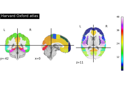
nilearn.plotting.plot_prob_atlasTo simply plot probabilistic atlases (4D images)
Notes
A small threshold is applied by default to eliminate numerical background noise.
For visualization, non-finite values found in passed ‘roi_img’ or ‘bg_img’ are set to zero.
Examples using nilearn.plotting.plot_roi
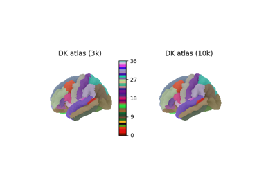
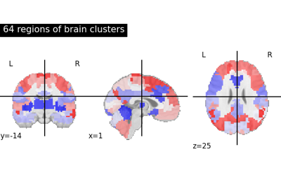
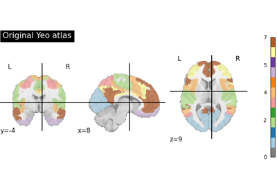
Visualizing multiscale functional brain parcellations
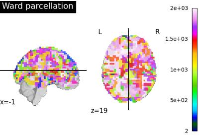
Clustering methods to learn a brain parcellation from fMRI
Computing a Region of Interest (ROI) mask manually