Glass brain plotting in nilearn (all options)

The first part of this example goes through different options of the plot_glass_brain function (including plotting negative values).

The second part goes through same options but selected of the same glass brain function but plotting is seen with contours.

See Plotting brain images for more plotting functionalities and Section 4.3 for more details about display objects in Nilearn.

Also, see load_sample_motor_activation_image for details about the plotting data and associated meta-data.

Load the data

We will use a motor activation contrast map distributed with Nilearn.

from nilearn import datasets

stat_img = datasets.load_sample_motor_activation_image()

# stat_img is just the name of the image file
stat_img

'/home/runner/work/nilearn/nilearn/.tox/doc/lib/python3.10/site-packages/nilearn/datasets/data/image_10426.nii.gz'

Demo glass brain plotting

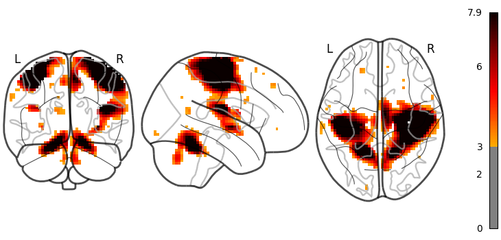
By default, plot_glass_brain uses a display mode called ‘ortho’ which results in three projections. It is equivalent to specify display_mode='ortho' in plot_glass_brain. Note that depending on the value of display_mode, different display objects are returned. Here, a OrthoProjector is returned.

from nilearn.plotting import plot_glass_brain, show

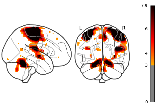
# Whole brain sagittal cuts and map is thresholded at 3

plot_glass_brain(stat_img, threshold=3)

<nilearn.plotting.displays._projectors.OrthoProjector object at 0x7f114e6083a0>

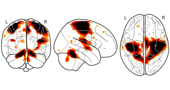
The same figure, without a colorbar, can be produced by setting colorbar=False.

plot_glass_brain(stat_img, threshold=3, colorbar=False)

<nilearn.plotting.displays._projectors.OrthoProjector object at 0x7f114e018d60>

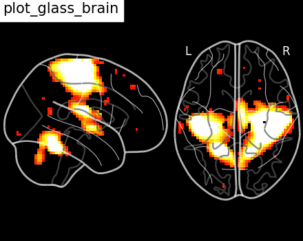
Here, we show how to set a black background, and we only view sagittal and axial projections by setting display_mode='xz', which returns a XZProjector.

plot_glass_brain(
    stat_img,
    title="plot_glass_brain",
    black_bg=True,
    display_mode="xz",
    threshold=3,
)

<nilearn.plotting.displays._projectors.XZProjector object at 0x7f114e633520>

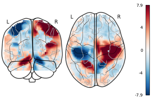
We can also plot the sign of the activation by setting plot_abs=False. Additionally, we only visualize coronal and axial projections by setting display_mode='yz' which returns a YZProjector.

plot_glass_brain(stat_img, threshold=0, plot_abs=False, display_mode="yz")

<nilearn.plotting.displays._projectors.YZProjector object at 0x7f115b8ddff0>

Setting plot_abs=True and display_mode='yx' (returns a YXProjector).

plot_glass_brain(stat_img, threshold=3, plot_abs=True, display_mode="yx")

<nilearn.plotting.displays._projectors.YXProjector object at 0x7f114e98a4d0>

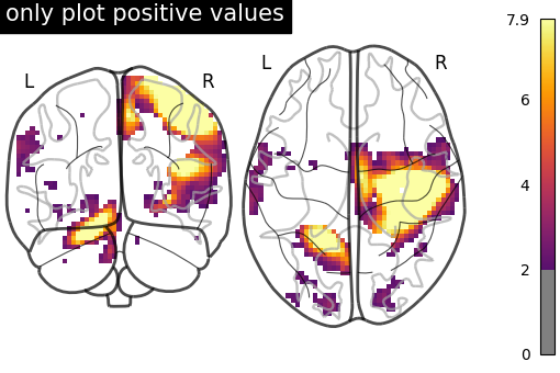
We can control the limits of the colormap and colorbar by setting vmin and vmax. Note that we use a non-diverging colormap here since the colorbar will not be centered around zero.

# only plot positive values
plot_glass_brain(
    stat_img,
    plot_abs=False,
    display_mode="yz",
    vmin=0,
    threshold=2,
    symmetric_cbar=False,
    cmap="inferno",
    title="only plot positive values",
)

<nilearn.plotting.displays._projectors.YZProjector object at 0x7f115c6106a0>

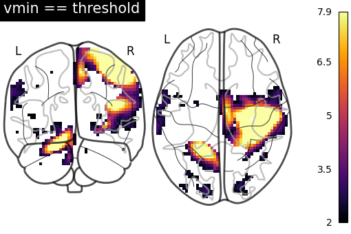
Here we set vmin to the threshold to use the full color range instead of losing colors due to the thresholding.

plot_glass_brain(
    stat_img,
    plot_abs=False,
    display_mode="yz",
    vmin=2,
    threshold=2,
    symmetric_cbar=False,
    cmap="inferno",
    title="vmin == threshold",
)

<nilearn.plotting.displays._projectors.YZProjector object at 0x7f114e2f8340>

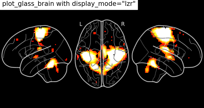
Different projections for the left and right hemispheres

In the previous section we saw a few projection modes, which are controlled by setting the argument display_mode of plot_glass_brain. In this section, we will show some additional possibilities. For example, setting display_mode='lzr' enables an hemispheric sagittal view. The display object returned is then a LZRProjector.

plot_glass_brain(
    stat_img,
    title='plot_glass_brain with display_mode="lzr"',
    black_bg=True,
    display_mode="lzr",
    threshold=3,
)

<nilearn.plotting.displays._projectors.LZRProjector object at 0x7f115b8521d0>

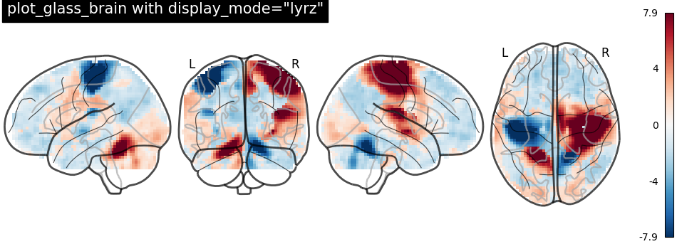
display_mode='lyrz' returns a LYRZProjector object.

plot_glass_brain(
    stat_img,
    threshold=0,
    title='plot_glass_brain with display_mode="lyrz"',
    plot_abs=False,
    display_mode="lyrz",
)

<nilearn.plotting.displays._projectors.LYRZProjector object at 0x7f114e3ff580>

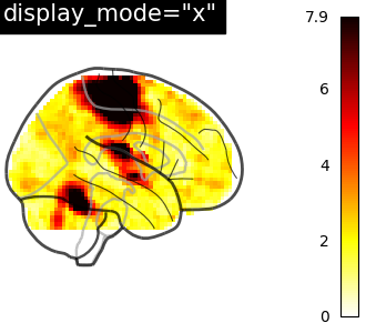
If you are only interested in single projections, you can set display_mode to ‘x’ (returns a XProjector), ‘y’ (returns a YProjector), ‘z’ (returns a ZProjector), ‘l’ (returns a LProjector), or ‘r’ (returns a RProjector).

plot_glass_brain(
    stat_img,
    threshold=0,
    title='display_mode="x"',
    plot_abs=True,
    display_mode="x",
)

<nilearn.plotting.displays._projectors.XProjector object at 0x7f115c6702b0>

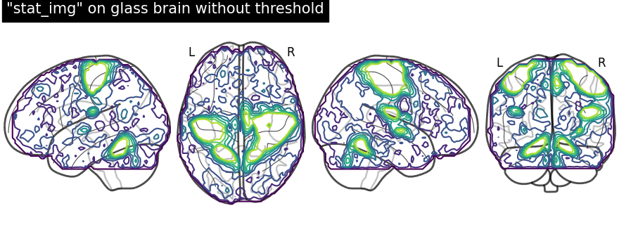
Contours and with fillings

The display objects returned by plot_glass_brain all inherit from the OrthoProjector and enable further customization of the figures.

In this example, we focus on using methods add_contours and title. First, we save the display object (here a LZRYProjector) into a variable named display. Note that we set the first argument to None since we want an empty glass brain to plot the statistical maps with add_contours.

display = plot_glass_brain(None, display_mode="lzry")
# Here, we project statistical maps
display.add_contours(stat_img)
# and add a title
display.title('"stat_img" on glass brain without threshold')

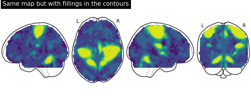
We can fill the contours by setting filled=True. Note that we are not specifying levels here

display = plot_glass_brain(None, display_mode="lzry")
# Here, we project statistical maps with filled=True
display.add_contours(stat_img, filled=True)
# and add a title
display.title("Same map but with fillings in the contours")

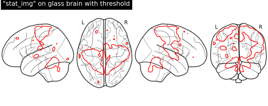
Here, we input a specific level (cut-off) in the statistical map. In other words, we are thresholding our statistical map.

We set the threshold using a parameter of method add_contours called levels which value is given as a list and we choose the color to be red.

display = plot_glass_brain(None, display_mode="lzry")
display.add_contours(stat_img, levels=[3.0], colors="r")
display.title('"stat_img" on glass brain with threshold')

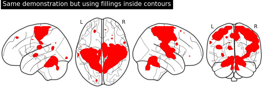
Plotting with same demonstration but fill the contours (by setting filled=True).

display = plot_glass_brain(None, display_mode="lzry")
display.add_contours(stat_img, filled=True, levels=[3.0], colors="r")
display.title("Same demonstration but using fillings inside contours")

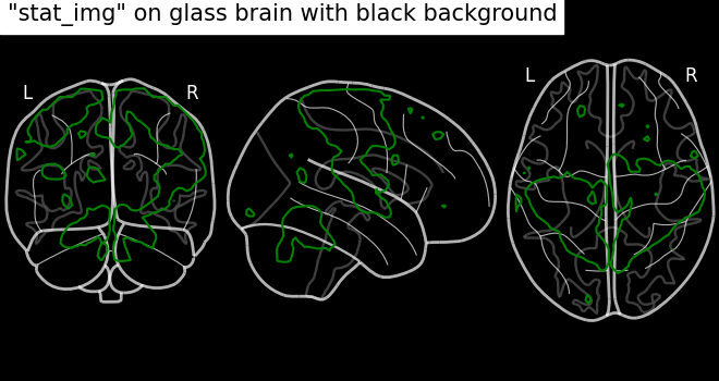
Plotting with black background, black_bg should be set to True through plot_glass_brain.

# We can set black background using black_bg=True
display = plot_glass_brain(None, black_bg=True)
display.add_contours(stat_img, levels=[3.0], colors="g")
display.title('"stat_img" on glass brain with black background')

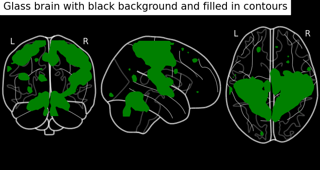
Black background plotting with filled in contours.

display = plot_glass_brain(None, black_bg=True)
display.add_contours(stat_img, filled=True, levels=[3.0], colors="g")
display.title("Glass brain with black background and filled in contours")

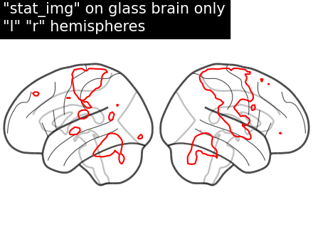
Contour projections in both hemispheres

The key argument to vary here is display_mode for hemispheric plotting. Here, we set display_mode='lr' for both hemispheric plots. Note that a LRProjector is returned.

display = plot_glass_brain(None, display_mode="lr")
display.add_contours(stat_img, levels=[3.0], colors="r")
display.title('"stat_img" on glass brain only\n"l" "r" hemispheres')

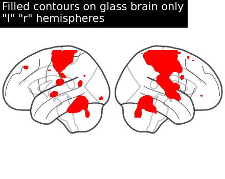
Filled contours in both hemispheric plotting, by adding filled=True.

display = plot_glass_brain(None, display_mode="lr")
display.add_contours(stat_img, filled=True, levels=[3.0], colors="r")
display.title('Filled contours on glass brain only\n"l" "r" hemispheres')

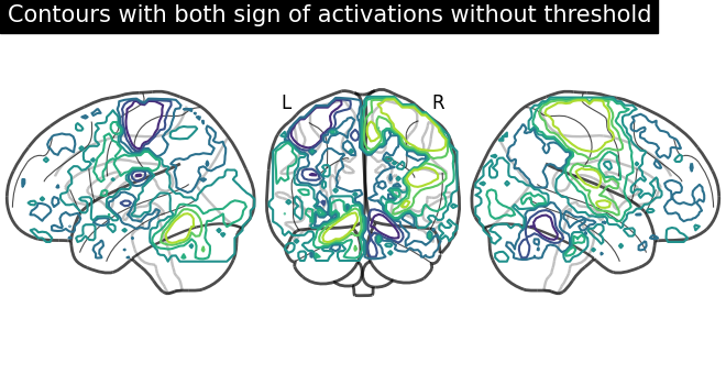
With positive and negative signs of activations with plot_abs in plot_glass_brain.

By default parameter plot_abs is True and sign of activations can be displayed by changing plot_abs to False. Note that we also specify display_mode='lyr' which returns a LYRProjector display object.

display = plot_glass_brain(None, plot_abs=False, display_mode="lyr")
display.add_contours(stat_img)
display.title("Contours with both sign of activations without threshold")

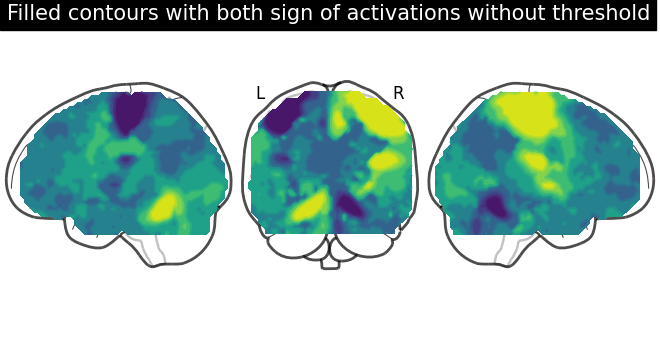
Now, adding filled=True to get positive and negative sign activations with fillings in the contours.

display = plot_glass_brain(None, plot_abs=False, display_mode="lyr")
display.add_contours(stat_img, filled=True)
display.title(
    "Filled contours with both sign of activations without threshold"
)

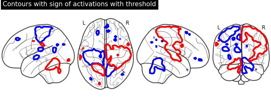
Displaying both signs (positive and negative) of activations with threshold meaning thresholding by adding an argument levels in method add_contours.

We give two values through the argument levels which corresponds to the thresholds of the contour we want to draw: One is positive and the other one is negative. We give a list of colors as argument to associate a different color to each contour. Additionally, we also choose to plot contours with thick line widths. For linewidths, one value would be enough so that same value is used for both contours.

import numpy as np

display = plot_glass_brain(None, plot_abs=False, display_mode="lzry")
display.add_contours(
    stat_img, levels=[-2.8, 3.0], colors=["b", "r"], linewidths=4.0
)
display.title("Contours with sign of activations with threshold")

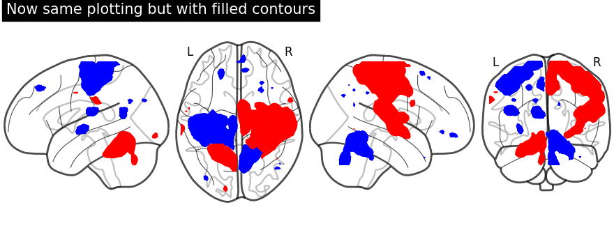
Same display demonstration as above but adding filled=True to get fillings inside the contours.

Unlike in previous plot, here we specify each sign at a time. We call negative values display first followed by positive values display.

First, we fetch our display object with same parameters used as above. Then, we plot negative sign of activation with levels given as negative activation value in a list. Upper bound should be kept to -infinity. Next, using the same display object, we plot positive sign of activation.

display = plot_glass_brain(None, plot_abs=False, display_mode="lzry")
display.add_contours(stat_img, filled=True, levels=[-np.inf, -2.8], colors="b")
display.add_contours(stat_img, filled=True, levels=[3.0], colors="r")
display.title("Now same plotting but with filled contours")
# Finally, displaying them
show()

Estimated memory usage: 99 MB