Note
Go to the end to download the full example code. or to run this example in your browser via Binder
Intro to GLM Analysis: a single-run, single-subject fMRI dataset
In this tutorial, we use a General Linear Model (GLM) to compare the fMRI signal during periods of auditory stimulation versus periods of rest.
Warning
The analysis described here is performed in the native space, directly on the original EPI scans without any spatial or temporal preprocessing. More sensitive results would likely be obtained on the corrected, spatially normalized and smoothed images.
Retrieving the data
Note
In this tutorial, we load the data using a data downloading
function. To input your own data, you will need to provide
a list of paths to your own files in the subject_data variable.
These should abide to the Brain Imaging Data Structure
(BIDS) organization.
from nilearn.datasets import fetch_spm_auditory

subject_data = fetch_spm_auditory()
[fetch_spm_auditory] Dataset directory found:
/home/runner/work/nilearn/nilearn/nilearn_data/spm_auditory
Inspecting the dataset
print paths of func image
'/home/runner/work/nilearn/nilearn/nilearn_data/spm_auditory/MoAEpilot/sub-01/func/sub-01_task-auditory_bold.nii'
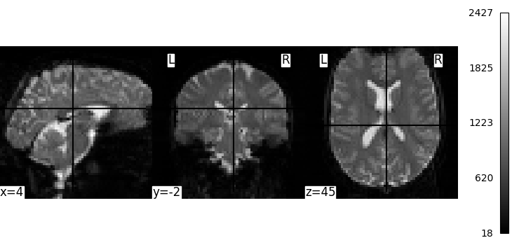
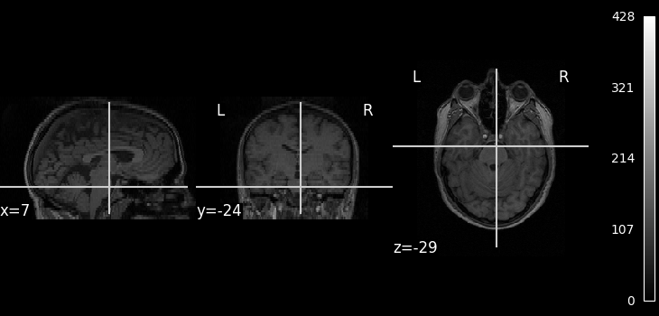
We can display the mean functional image and the subject’s anatomy:
from nilearn.image import mean_img
from nilearn.plotting import plot_anat, plot_img, plot_stat_map, show

fmri_img = subject_data.func
mean_img = mean_img(subject_data.func[0])
plot_img(mean_img, cbar_tick_format="%i")

plot_anat(subject_data.anat, cbar_tick_format="%i")

show()
Specifying the experimental paradigm
We must now provide a description of the experiment, that is, define the timing of the auditory stimulation and rest periods. This is typically provided in an events.tsv file. The path of this file is provided in the dataset.
import pandas as pd

events = pd.read_table(subject_data.events)
events
Performing the GLM analysis
It is now time to create and estimate a FirstLevelModel object,
that will generate the design matrix
using the information provided by the events object.
from nilearn.glm.first_level import FirstLevelModel
Parameters of the first-level model
t_r=7(s)is the time of repetition of acquisitionsnoise_model='ar1'specifies the noise covariance model: a lag-1 dependencestandardize=Falsemeans that we do not want to rescale the time series to mean 0, variance 1hrf_model='spm'means that we rely on the SPM “canonical hrf” model (without time or dispersion derivatives)drift_model='cosine'means that we model the signal drifts as slow oscillating time functionshigh_pass=0.01(Hz) defines the cutoff frequency (inverse of the time period).
fmri_glm = FirstLevelModel(
    t_r=subject_data.t_r,
    noise_model="ar1",
    standardize=False,
    hrf_model="spm",
    drift_model="cosine",
    high_pass=0.01,
    verbose=1,
)
Note
When viewing an Nilearn estimator in a notebook (or more generally on an HTML page like here) you get an expandable ‘Parameters’ section where the parameters that have different values from their default are highlighted in orange. If you are using a version of scikit-learn >= 1.8.0 you will also get access to the ‘docstring’ description of each parameter.
Now that we have specified the model, we can run it on the fMRI image
Note
After fitting, the HTML representation of the estimator looks different than before fitting.
\[FirstLevelModel.fit] Computing run 1 out of 1 runs (go take a coffee, a big
one).
\[FirstLevelModel.fit] Performing mask computation.
\[FirstLevelModel.fit] Masking took 0 seconds.
\[FirstLevelModel.fit] Performing GLM computation.
\[FirstLevelModel.fit] GLM took 1 seconds.
\[FirstLevelModel.fit] Computation of 1 runs done in 00 HR 00 MIN 02 SEC.
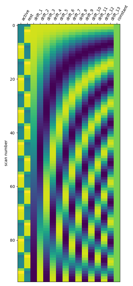
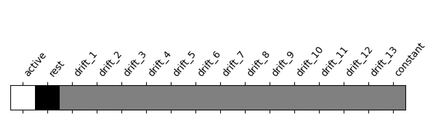
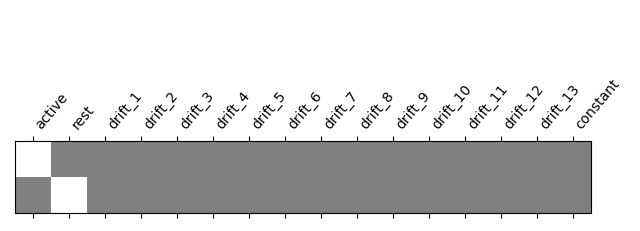
One can inspect the design matrix (rows represent time, and columns contain the predictors).
Formally, we have taken the first design matrix, because the model is implictily meant to for multiple runs.
from nilearn.plotting import plot_design_matrix

plot_design_matrix(design_matrix)

show()
Save the design matrix image to disk first create a directory where you want to write the images
from pathlib import Path

output_dir = Path.cwd() / "results" / "plot_single_subject_single_run"
output_dir.mkdir(exist_ok=True, parents=True)
print(f"Output will be saved to: {output_dir}")

plot_design_matrix(design_matrix, output_file=output_dir / "design_matrix.png")
Output will be saved to: /home/runner/work/nilearn/nilearn/examples/00_tutorials/results/plot_single_subject_single_run

<Axes: label='conditions', ylabel='scan number'>
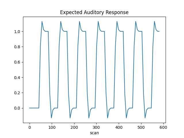
The first column contains the expected response profile of regions which are sensitive to the auditory stimulation. Let’s plot this first column
import matplotlib.pyplot as plt

plt.plot(design_matrix["listening"])
plt.xlabel("scan")
plt.title("Expected Auditory Response")

show()
Detecting voxels with significant effects
To access the estimated coefficients (Betas of the GLM model), we created contrast with a single ‘1’ in each of the columns: The role of the contrast is to select some columns of the model –and potentially weight them– to study the associated statistics. So in a nutshell, a contrast is a weighted combination of the estimated effects. Here we can define canonical contrasts that just consider the effect of the stimulation in isolation.
Note
Here the baseline is implicit, so passing a value of 1
for the first column will give contrast for: listening > rest
import numpy as np

n_regressors = design_matrix.shape[1]
activation = np.zeros(n_regressors)
activation[0] = 1
Let’s look at it: plot the coefficients of the contrast, indexed by the names of the columns of the design matrix.
from nilearn.plotting import plot_contrast_matrix

plot_contrast_matrix(contrast_def=activation, design_matrix=design_matrix)
<Axes: label='conditions'>
Below, we compute the ‘estimated effect’. It is in BOLD signal unit, but has no statistical guarantees, because it does not take into account the associated variance.
eff_map = fmri_glm.compute_contrast(activation, output_type="effect_size")
In order to get statistical significance, we form a t-statistic, and directly convert it into z-scale. The z-scale means that the values are scaled to match a standard Gaussian distribution (mean=0, variance=1), across voxels, if there were no effects in the data.
z_map = fmri_glm.compute_contrast(activation, output_type="z_score")
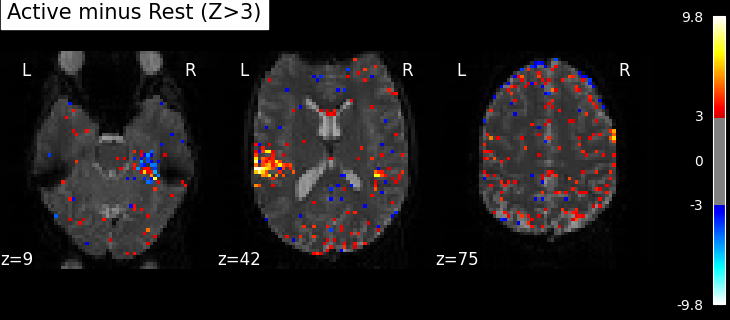
Plot thresholded z scores map
We display it on top of the average functional image of the series (could be the anatomical image of the subject). We use arbitrarily a threshold of 3.0 in z-scale. We’ll see later how to use corrected thresholds. We will show 3 axial views, with display_mode=’z’ and cut_coords=3.
plotting_config = {
    "bg_img": mean_img,
    "display_mode": "z",
    "cut_coords": 3,
    "black_bg": True,
}
plot_stat_map(
    z_map,
    threshold=3,
    title="listening > rest (|Z|>3)",
    figure=plt.figure(figsize=(10, 4)),
    **plotting_config,
)
show()

Note
Notice how the visualizations above shows both ‘activated’ voxels with Z > 3, as well as ‘deactivated’ voxels with Z < -3. In the rest of this example we will show only the activate voxels by using one-sided tests.
Statistical significance testing
One should worry about the statistical validity of the procedure: here we used an arbitrary threshold of 3.0 but the threshold should provide some guarantees on the risk of false detections (aka type-1 errors in statistics). One suggestion is to control the false positive rate (fpr, denoted by alpha) at a certain level, e.g. 0.001: this means that there is 0.1% chance of declaring an inactive voxel, active.
from nilearn.glm import threshold_stats_img

clean_map, threshold = threshold_stats_img(
    z_map,
    alpha=0.001,
    height_control="fpr",
    two_sided=False,  # using a one-sided test
)
# Let's use a sequential colormap as we will only display positive values.
plotting_config["cmap"] = "inferno"
plot_stat_map(
    clean_map,
    threshold=threshold,
    title=(
        f"listening > rest (Uncorrected p<0.001; threshold: {threshold:.3f})"
    ),
    figure=plt.figure(figsize=(10, 4)),
    **plotting_config,
)
show()
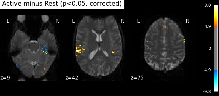
The problem is that with this you expect 0.001 * n_voxels to show up while they’re not active — tens to hundreds of voxels. A more conservative solution is to control the family wise error rate, i.e. the probability of making only one false detection, say at 5%. For that we use the so-called Bonferroni correction.
clean_map, threshold = threshold_stats_img(
    z_map, alpha=0.05, height_control="bonferroni", two_sided=False
)
plot_stat_map(
    clean_map,
    threshold=threshold,
    title=(
        "listening > rest (p<0.05 Bonferroni-corrected, "
        f"threshold: {threshold:.3f})"
    ),
    figure=plt.figure(figsize=(10, 4)),
    **plotting_config,
)
show()
This is quite conservative indeed! A popular alternative is to control the expected proportion of false discoveries among detections. This is called the False discovery rate.
clean_map, threshold = threshold_stats_img(
    z_map, alpha=0.05, height_control="fdr", two_sided=False
)
plot_stat_map(
    clean_map,
    threshold=threshold,
    title=(
        f"listening > rest (p<0.05 FDR-corrected; threshold: {threshold:.3f})"
    ),
    figure=plt.figure(figsize=(10, 4)),
    **plotting_config,
)
show()
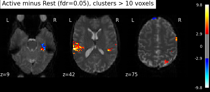
Finally people like to discard isolated voxels (aka “small clusters”) from these images. It is possible to generate a thresholded map with small clusters removed by providing a cluster_threshold argument. Here clusters smaller than 10 voxels will be discarded.
clean_map, threshold = threshold_stats_img(
    z_map,
    alpha=0.05,
    height_control="fdr",
    cluster_threshold=10,
    two_sided=False,
)
plot_stat_map(
    clean_map,
    threshold=threshold,
    title=(
        "listening > rest "
        f"(p<0.05 FDR-corrected; threshold: {threshold:.3f}; "
        "clusters > 10 voxels)"
    ),
    figure=plt.figure(figsize=(10, 4)),
    **plotting_config,
)
show()
We can save the effect and zscore maps to the disk.
z_map.to_filename(output_dir / "listening_gt_rest_z_map.nii.gz")
eff_map.to_filename(output_dir / "listening_gt_rest_eff_map.nii.gz")
We can furthermore extract and report the found positions in a table.
See also
This function does not report any named anatomical location for the clusters. To get the names of the location of the clusters according to one or several atlases, we recommend using the atlasreader package.
from nilearn.reporting import get_clusters_table

table = get_clusters_table(
    z_map, stat_threshold=threshold, cluster_threshold=20
)
table
This table can be saved for future use.
table.to_csv(output_dir / "table.csv")
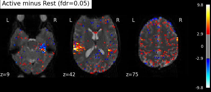
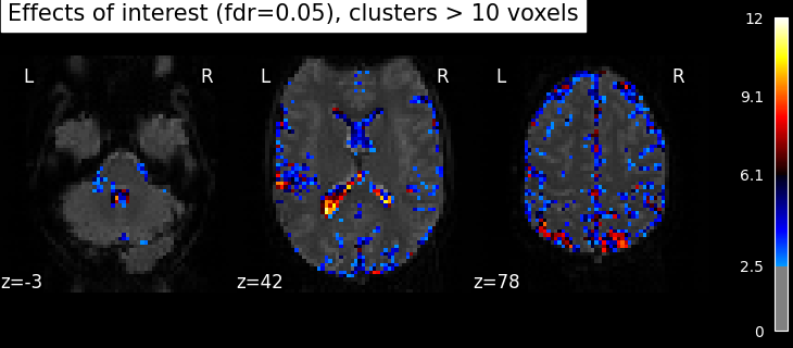
Performing an F-test
“listening > rest” is a typical t test: condition versus baseline. Another popular type of test is an F test in which one seeks whether a certain combination of conditions (possibly two-, three- or higher-dimensional) explains a significant proportion of the signal. Here one might for instance test which voxels are well explained by the combination of more active or less active than rest.
Note
As opposed to t-tests, the beta images produced by of F-tests only contain positive values.
Specify the contrast and compute the corresponding map. Actually, the contrast specification is done exactly the same way as for t-contrasts.
z_map = fmri_glm.compute_contrast(
    activation,
    output_type="z_score",
    stat_type="F",  # set stat_type to 'F' to perform an F test
)
Note that the statistic has been converted to a z-variable, which makes it easier to represent it.
clean_map, threshold = threshold_stats_img(
    z_map,
    alpha=0.05,
    height_control="fdr",
    cluster_threshold=10,
    two_sided=False,
)
plot_stat_map(
    clean_map,
    threshold=threshold,
    title="Effects of interest (fdr=0.05), clusters > 10 voxels",
    figure=plt.figure(figsize=(10, 4)),
    **plotting_config,
)
show()
Total running time of the script: (0 minutes 11.091 seconds)
Estimated memory usage: 474 MB