Clustering methods to learn a brain parcellation from fMRI

We use spatially-constrained Ward-clustering, KMeans, Hierarchical KMeans and Recursive Neighbor Agglomeration (ReNA) to create a set of parcels.

In a high dimensional regime, these methods can be interesting to create a ‘compressed’ representation of the data, replacing the data in the fMRI images by mean signals on the parcellation, which can subsequently be used for statistical analysis or machine learning.

Also, these methods can be used to learn functional connectomes and subsequently for classification tasks or to analyze data at a local level.

See also

An empirical comparison on which clustering method to use can be found in Thirion et al.[1].

This parcellation may be useful in a supervised learning, see for instance Michel et al.[2].

The big picture discussion corresponding to this example can be found in the documentation section Clustering to parcellate the brain in regions.

Download a brain development fMRI dataset

We download one subject of the movie watching dataset.

import numpy as np

from nilearn import datasets

dataset = datasets.fetch_development_fmri(n_subjects=1)

# print basic information on the dataset
print(f"First subject functional nifti image (4D) is at: {dataset.func[0]}")

[fetch_development_fmri] Dataset directory found: /home/runner/work/nilearn/nilearn/nilearn_data/development_fmri
First subject functional nifti image (4D) is at: /home/runner/work/nilearn/nilearn/nilearn_data/development_fmri/sub-pixar123_task-pixar_space-MNI152NLin2009cAsym_desc-preproc_bold.nii.gz

Brain parcellation with Ward clustering

Transforming list of images to data matrix and building brain parcellations can all be done at once using Parcellation objects.

Note

Computing ward for the first time will be long… Time spent can be measured using time.

We build parameters of our own for this object with parameters related to masking, caching and defining number of clusters and specific parcellation method.

import time

from nilearn.regions import Parcellations

start = time.time()
ward = Parcellations(
    method="ward",
    n_parcels=1000,
    smoothing_fwhm=2.0,
    memory="nilearn_cache",
    memory_level=1,
    verbose=1,
)
# Call fit on functional dataset: single subject (fewer samples).
ward.fit(dataset.func)

[Parcellations.fit] Loading data
[Parcellations.fit] computing ward
________________________________________________________________________________
[Memory] Calling nilearn.regions.parcellations._estimator_fit...
_estimator_fit(array([[-0.002154, ...,  0.002661],
       ...,
       [ 0.007053, ..., -0.007877]]),
AgglomerativeClustering(connectivity=<24256x24256 sparse matrix of type '<class 'numpy.int64'>'
        with 162682 stored elements in COOrdinate format>,
                        memory=Memory(location=nilearn_cache/joblib),
                        n_clusters=1000))
________________________________________________________________________________
[Memory] Calling sklearn.cluster._agglomerative.ward_tree...
ward_tree(array([[-0.002154, ...,  0.007053],
       ...,
       [ 0.002661, ..., -0.007877]]), connectivity=<24256x24256 sparse matrix of type '<class 'numpy.int64'>'
        with 162682 stored elements in COOrdinate format>, n_clusters=1000, return_distance=False)
________________________________________________________ward_tree - 1.8s, 0.0min
____________________________________________________estimator_fit - 1.9s, 0.0min

Parcellations(memory='nilearn_cache', memory_level=1, method='ward',
              n_parcels=1000, smoothing_fwhm=2.0, verbose=1)

In a Jupyter environment, please rerun this cell to show the HTML representation or trust the notebook.
On GitHub, the HTML representation is unable to render, please try loading this page with nbviewer.org.

print(f"Ward agglomeration 1000 clusters: {time.time() - start:.2f}s")

Ward agglomeration 1000 clusters: 5.01s

We now compute ward clustering with 2000 clusters and compare the time spent for computing with 1000 clusters to see the benefits of caching.

We instantiate a new instance with n_parcels=2000 this time.

start = time.time()
ward = Parcellations(
    method="ward",
    n_parcels=2000,
    smoothing_fwhm=2.0,
    memory="nilearn_cache",
    memory_level=1,
    verbose=1,
)
ward.fit(dataset.func)

[Parcellations.fit] Loading data
[Parcellations.fit] computing ward
________________________________________________________________________________
[Memory] Calling nilearn.regions.parcellations._estimator_fit...
_estimator_fit(array([[-0.002154, ...,  0.002661],
       ...,
       [ 0.007053, ..., -0.007877]]),
AgglomerativeClustering(connectivity=<24256x24256 sparse matrix of type '<class 'numpy.int64'>'
        with 162682 stored elements in COOrdinate format>,
                        memory=Memory(location=nilearn_cache/joblib),
                        n_clusters=2000))
________________________________________________________________________________
[Memory] Calling sklearn.cluster._agglomerative.ward_tree...
ward_tree(array([[-0.002154, ...,  0.007053],
       ...,
       [ 0.002661, ..., -0.007877]]), connectivity=<24256x24256 sparse matrix of type '<class 'numpy.int64'>'
        with 162682 stored elements in COOrdinate format>, n_clusters=2000, return_distance=False)
________________________________________________________ward_tree - 1.9s, 0.0min
____________________________________________________estimator_fit - 1.9s, 0.0min

Parcellations(memory='nilearn_cache', memory_level=1, method='ward',
              n_parcels=2000, smoothing_fwhm=2.0, verbose=1)

In a Jupyter environment, please rerun this cell to show the HTML representation or trust the notebook.
On GitHub, the HTML representation is unable to render, please try loading this page with nbviewer.org.

We can observe that although the number of clusters doubles, computation takes less time.

print(f"Ward agglomeration 2000 clusters: {time.time() - start:.2f}s")

Ward agglomeration 2000 clusters: 4.23s

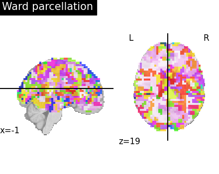
Visualize: Brain parcellation (Ward)

First, we display the parcellation of the brain image stored in attribute labels_img_.

from nilearn import plotting

ward_labels_img = ward.labels_img_

first_plot = plotting.plot_roi(
    ward_labels_img, title="Ward parcellation", display_mode="xz"
)

plotting.show()

# We grab the cut coordinates from this plot to use as a common for all plots.
cut_coords = first_plot.cut_coords

Compressed representation of Ward clustering

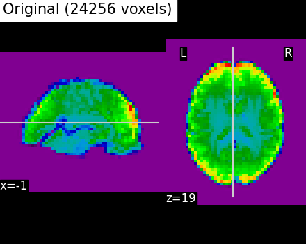
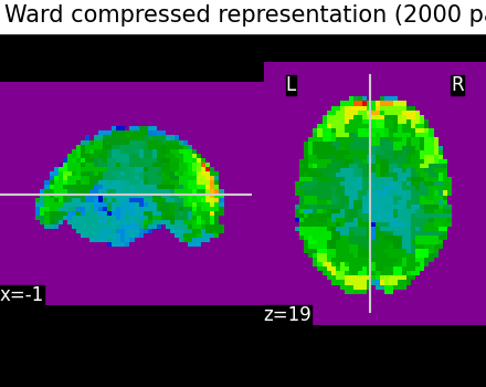
Second, we illustrate the effect of the clustering on the signal. We show the original data, and the approximation provided by the clustering by averaging the signal on each parcel.

# Grab the number of voxels from attribute mask image (mask_img_).
from nilearn.image import get_data

original_voxels = np.sum(get_data(ward.mask_img_))

# Compute mean over time on the functional image to use the mean
# image for compressed representation comparisons
from nilearn.image import mean_img

mean_func_img = mean_img(dataset.func[0])

# Compute common vmin and vmax
vmin = np.min(get_data(mean_func_img))
vmax = np.max(get_data(mean_func_img))

plotting.plot_epi(
    mean_func_img,
    cut_coords=cut_coords,
    title=f"Original ({int(original_voxels)} voxels)",
    vmax=vmax,
    vmin=vmin,
    display_mode="xz",
)

<nilearn.plotting.displays._slicers.XZSlicer object at 0x7faa94db3e50>

A reduced dataset can be created by taking the parcel-level average.

Parcellation objects with any method have the opportunity to use a transform call that modifies input features. Here it reduces their dimension. Note that we fit before calling a transform so that average signals can be created on the brain parcellation with fit.

fmri_reduced = ward.transform(dataset.func)

# Display the corresponding data compressed
# using the previous parcellation.
from nilearn.image import index_img

fmri_compressed = ward.inverse_transform(fmri_reduced)

plotting.plot_epi(
    index_img(fmri_compressed, 0),
    cut_coords=cut_coords,
    title=f"Ward compressed representation ({ward.n_parcels} parcels)",
    vmin=vmin,
    vmax=vmax,
    display_mode="xz",
)

plotting.show()

[Parcellations.wrapped] Loading data from <nibabel.nifti1.Nifti1Image object at 0x7faa94c02790>
[Parcellations.wrapped] Loading mask from <nibabel.nifti1.Nifti1Image object at 0x7faa94d42450>
[Parcellations.wrapped] Loading regions from <nibabel.nifti1.Nifti1Image object at 0x7faa6a0bfb50>
[Parcellations.wrapped] Finished fit
________________________________________________________________________________
[Memory] Calling nilearn.maskers.base_masker.filter_and_extract...
filter_and_extract(<nibabel.nifti1.Nifti1Image object at 0x7faa94c02790>, <nilearn.maskers.nifti_labels_masker._ExtractionFunctor object at 0x7faaa68a2310>,
{ 'background_label': 0,
  'clean_args': None,
  'clean_kwargs': {},
  'cmap': None,
  'detrend': False,
  'dtype': None,
  'high_pass': None,
  'high_variance_confounds': False,
  'labels': None,
  'labels_img': <nibabel.nifti1.Nifti1Image object at 0x7faa6a0bfb50>,
  'low_pass': None,
  'lut': None,
  'mask_img': <nibabel.nifti1.Nifti1Image object at 0x7faa94d42450>,
  'reports': True,
  'smoothing_fwhm': 2.0,
  'standardize': None,
  'standardize_confounds': True,
  'strategy': 'mean',
  't_r': None,
  'target_affine': None,
  'target_shape': None}, confounds=None, sample_mask=None, memory=Memory(location=nilearn_cache/joblib), memory_level=1, verbose=1, sklearn_output_config=None)
[Parcellations.wrapped] Loading data from <nibabel.nifti1.Nifti1Image object at 0x7faa94c02790>
[Parcellations.wrapped] Smoothing images
[Parcellations.wrapped] Extracting region signals
[Parcellations.wrapped] Cleaning extracted signals
_______________________________________________filter_and_extract - 0.8s, 0.0min

As you can see, this approximation is almost good, although there are only 2000 parcels instead of the original 60000 voxels.

Brain parcellation with KMeans Clustering

We use the same approach as building parcellation using Ward clustering. But, in the range of a small number of clusters, it is most likely that we want to use standardization. Indeed with standardization and smoothing, the clusters will form as regions.

This next parcellation uses method='kmeans' for KMeans clustering with 10mm smoothing and standardization.

start = time.time()
kmeans = Parcellations(
    method="kmeans",
    n_parcels=50,
    smoothing_fwhm=10.0,
    standardize="zscore_sample",
    memory="nilearn_cache",
    memory_level=1,
    verbose=1,
)
# Call fit on functional dataset: single subject (fewer samples).
kmeans.fit(dataset.func)

[Parcellations.fit] Loading data
[Parcellations.fit] computing kmeans
________________________________________________________________________________
[Memory] Calling nilearn.regions.parcellations._estimator_fit...
_estimator_fit(array([[ 0.004934, ..., -0.015396],
       ...,
       [-0.003247, ..., -0.001756]]),
MiniBatchKMeans(n_clusters=50, n_init=3, random_state=0))
____________________________________________________estimator_fit - 0.2s, 0.0min

Parcellations(memory='nilearn_cache', memory_level=1, method='kmeans',
              smoothing_fwhm=10.0, standardize='zscore_sample', verbose=1)

In a Jupyter environment, please rerun this cell to show the HTML representation or trust the notebook.
On GitHub, the HTML representation is unable to render, please try loading this page with nbviewer.org.

print(f"KMeans clusters: {time.time() - start:.2f}s")

KMeans clusters: 3.47s

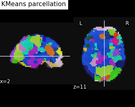
Visualize: Brain parcellation (KMeans)

We display the parcellation of the brain image stored in attribute labels_img_.

kmeans_labels_img = kmeans.labels_img_

display = plotting.plot_roi(
    kmeans_labels_img,
    mean_func_img,
    cut_coords=cut_coords,
    title="KMeans parcellation",
    display_mode="xz",
)

plotting.show()

Brain parcellation with Hierarchical KMeans Clustering

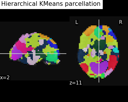
As the number of images from which we try to create clusters grows, voxels display more and more specific activity patterns causing KMeans clusters to be very unbalanced with a few big clusters and many voxels left as singletons.

Hierarchical Kmeans algorithm is tailored to enforce more balanced clusterings. To do this, Hierarchical Kmeans does a first Kmeans clustering in square root of n_parcels. In a second step, it clusters voxels inside each of these parcels in m pieces with m adapted to the size of the cluster in order to have n balanced clusters in the end.

This object uses method='hierarchical_kmeans' for Hierarchical KMeans clustering and 10mm smoothing and standardization to compare with the previous method.

start = time.time()
hkmeans = Parcellations(
    method="hierarchical_kmeans",
    n_parcels=50,
    smoothing_fwhm=10,
    standardize="zscore_sample",
    memory="nilearn_cache",
    memory_level=1,
    verbose=1,
)
# Call fit on functional dataset: single subject (fewer samples).
hkmeans.fit(dataset.func)

[Parcellations.fit] Loading data
[Parcellations.fit] computing hierarchical_kmeans
________________________________________________________________________________
[Memory] Calling nilearn.regions.parcellations._estimator_fit...
_estimator_fit(array([[ 0.004934, ..., -0.015396],
       ...,
       [-0.003247, ..., -0.001756]]),
HierarchicalKMeans(n_clusters=50), 'hierarchical_kmeans')
____________________________________________________estimator_fit - 0.7s, 0.0min

Parcellations(memory='nilearn_cache', memory_level=1,
              method='hierarchical_kmeans', smoothing_fwhm=10,
              standardize='zscore_sample', verbose=1)

In a Jupyter environment, please rerun this cell to show the HTML representation or trust the notebook.
On GitHub, the HTML representation is unable to render, please try loading this page with nbviewer.org.

Visualize: Brain parcellation (Hierarchical KMeans)

We display the parcellation of brain image stored in attribute labels_img_.

hkmeans_labels_img = hkmeans.labels_img_

plotting.plot_roi(
    hkmeans_labels_img,
    mean_func_img,
    title="Hierarchical KMeans parcellation",
    display_mode="xz",
    cut_coords=display.cut_coords,
)

plotting.show()

Compare Hierarchical Kmeans clusters with those from Kmeans

To compare those, we’ll first count how many voxels are contained in each of the 50 clusters for both algorithms and compare their cluster size distributions. Hierarchical KMeans should give clusters closer to average (600 here) than KMeans.

# First count how many voxels have each label
# (except 0 which is the background).
_, kmeans_counts = np.unique(get_data(kmeans_labels_img), return_counts=True)

_, hkmeans_counts = np.unique(get_data(hkmeans_labels_img), return_counts=True)

voxel_ratio = np.round(np.sum(kmeans_counts[1:]) / 50)

If all voxels not in background were balanced between clusters …

print(f"... each cluster should contain {voxel_ratio} voxels")

... each cluster should contain 485.0 voxels

Let’s plot clusters’ size distributions for both algorithms.

You can just skip the plotting code, the important part is the figure.

import matplotlib.pyplot as plt
from matplotlib import patches, ticker

bins = np.concatenate(
    [
        np.linspace(0, 500, 11),
        np.linspace(600, 2000, 15),
        np.linspace(3000, 10000, 8),
    ]
)
fig, axes = plt.subplots(
    nrows=2, sharex=True, gridspec_kw={"height_ratios": [4, 1]}
)
plt.semilogx()
axes[0].hist(kmeans_counts[1:], bins, color="blue")
axes[1].hist(hkmeans_counts[1:], bins, color="green")
axes[0].set_ylim(0, 16)
axes[1].set_ylim(4, 0)
axes[1].xaxis.set_major_formatter(ticker.ScalarFormatter())
axes[1].yaxis.set_label_coords(-0.08, 2)
fig.subplots_adjust(hspace=0)
plt.xlabel("Number of voxels (log)", fontsize=12)
plt.ylabel("Number of clusters", fontsize=12)
handles = [
    patches.Rectangle((0, 0), 1, 1, color=c, ec="k") for c in ["blue", "green"]
]
labels = ["Kmeans", "Hierarchical Kmeans"]
fig.legend(handles, labels, loc=(0.5, 0.8))

plotting.show()

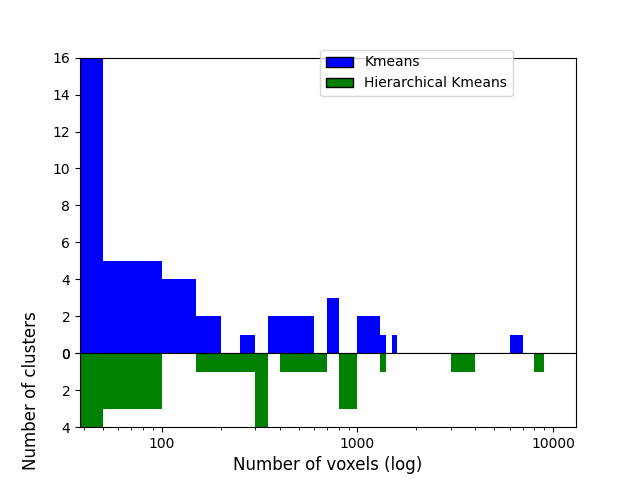
As we can see, half of the 50 KMeans clusters contain less than 100 voxels whereas three contain several thousands voxels. Hierarchical KMeans yield better balanced clusters, with a significant proportion of them containing hundreds to thousands of voxels.

Brain parcellation with ReNA Clustering

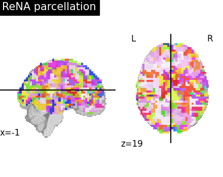
One interesting algorithmic property of ReNA is that it is very fast for a large number of parcels (notably faster than Ward). As before, the parcellation is done with a Parcellations object. The spatial constraints are implemented inside the Parcellations object.

More about ReNA clustering algorithm in the original paper (Hoyos-Idrobo et al.[3]).

start = time.time()
rena = Parcellations(
    method="rena",
    n_parcels=5000,
    smoothing_fwhm=2.0,
    scaling=True,
    memory="nilearn_cache",
    memory_level=1,
    verbose=1,
)

rena.fit_transform(dataset.func)

[Parcellations.wrapped] Loading data
[Parcellations.wrapped] computing rena
________________________________________________________________________________
[Memory] Calling nilearn.regions.parcellations._estimator_fit...
_estimator_fit(array([[-0.002154, ...,  0.002661],
       ...,
       [ 0.007053, ..., -0.007877]]),
ReNA(mask_img=<nibabel.nifti1.Nifti1Image object at 0x7faabe9b4050>,
     memory=Memory(location=nilearn_cache/joblib), n_clusters=5000,
     scaling=True),
'rena')
________________________________________________________________________________
[Memory] Calling nilearn.regions.rena_clustering.recursive_neighbor_agglomeration...
recursive_neighbor_agglomeration(array([[-0.002154, ...,  0.002661],
       ...,
       [ 0.007053, ..., -0.007877]]),
<nibabel.nifti1.Nifti1Image object at 0x7faa94ccdf10>, 5000, n_iter=10, threshold=1e-07, verbose=0)
_________________________________recursive_neighbor_agglomeration - 0.4s, 0.0min
____________________________________________________estimator_fit - 0.4s, 0.0min
[Parcellations.wrapped] Loading data from <nibabel.nifti1.Nifti1Image object at 0x7faa96863d90>
[Parcellations.wrapped] Loading mask from <nibabel.nifti1.Nifti1Image object at 0x7faa7122e6d0>
[Parcellations.wrapped] Loading regions from <nibabel.nifti1.Nifti1Image object at 0x7faac0f3e4d0>
[Parcellations.wrapped] Finished fit
________________________________________________________________________________
[Memory] Calling nilearn.maskers.base_masker.filter_and_extract...
filter_and_extract(<nibabel.nifti1.Nifti1Image object at 0x7faa96863d90>, <nilearn.maskers.nifti_labels_masker._ExtractionFunctor object at 0x7faabe627810>,
{ 'background_label': 0,
  'clean_args': None,
  'clean_kwargs': {},
  'cmap': None,
  'detrend': False,
  'dtype': None,
  'high_pass': None,
  'high_variance_confounds': False,
  'labels': None,
  'labels_img': <nibabel.nifti1.Nifti1Image object at 0x7faac0f3e4d0>,
  'low_pass': None,
  'lut': None,
  'mask_img': <nibabel.nifti1.Nifti1Image object at 0x7faa7122e6d0>,
  'reports': True,
  'smoothing_fwhm': 2.0,
  'standardize': None,
  'standardize_confounds': True,
  'strategy': 'mean',
  't_r': None,
  'target_affine': None,
  'target_shape': None}, confounds=None, sample_mask=None, memory=Memory(location=nilearn_cache/joblib), memory_level=1, verbose=1, sklearn_output_config=None)
[Parcellations.wrapped] Loading data from <nibabel.nifti1.Nifti1Image object at 0x7faa96863d90>
[Parcellations.wrapped] Smoothing images
[Parcellations.wrapped] Extracting region signals
[Parcellations.wrapped] Cleaning extracted signals
_______________________________________________filter_and_extract - 0.9s, 0.0min

array([[567.56117516, 569.00961211, 311.45420291, ..., 488.61132354,
        478.97656576, 299.90263484],
       [563.70982242, 569.00953865, 307.12138701, ..., 482.83444135,
        476.08827157, 299.90250262],
       [563.70979304, 569.49097978, 307.12140905, ..., 484.75997081,
        478.97669797, 294.12582611],
       ...,
       [575.26417445, 573.34243535, 331.67389291, ..., 482.83432383,
        476.08827157, 302.79101718],
       [579.11488078, 572.86082528, 328.78540039, ..., 482.83441197,
        473.19993331, 294.12582611],
       [569.48711596, 570.93531051, 328.78540039, ..., 480.90876499,
        476.0882275 , 305.67944358]])

print(f"ReNA 5000 clusters: {time.time() - start:.2f}s")

ReNA 5000 clusters: 3.83s

Visualize: Brain parcellation (ReNA)

We display the parcellation of the brain image stored in attribute labels_img_.

rena_labels_img = rena.labels_img_

plotting.plot_roi(
    ward_labels_img,
    title="ReNA parcellation",
    display_mode="xz",
    cut_coords=cut_coords,
)

plotting.show()

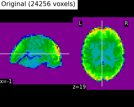
Compressed representation of ReNA clustering

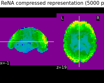
We illustrate the effect of clustering on the signal. We show the original data, and the approximation provided by the clustering by averaging the signal on each parcel.

We can then compare the results with the compressed representation obtained with Ward.

# Display the original data
plotting.plot_epi(
    mean_func_img,
    cut_coords=cut_coords,
    title=f"Original ({int(original_voxels)} voxels)",
    vmax=vmax,
    vmin=vmin,
    display_mode="xz",
)

<nilearn.plotting.displays._slicers.XZSlicer object at 0x7faa6a6a6a90>

A reduced data can be created by taking the parcel-level average: Note that, as many scikit-learn objects, the rena object exposes a transform method that modifies input features. Here it reduces their dimension. However, the data are in one single large 4D image, we need to use index_img to do the split easily:

fmri_reduced_rena = rena.transform(dataset.func)

# Display the corresponding data compression using the parcellation
compressed_img_rena = rena.inverse_transform(fmri_reduced_rena)

plotting.plot_epi(
    index_img(compressed_img_rena, 0),
    cut_coords=cut_coords,
    title=f"ReNA compressed representation ({rena.n_parcels} parcels)",
    vmin=vmin,
    vmax=vmax,
    display_mode="xz",
)

plotting.show()

[Parcellations.wrapped] Loading data from <nibabel.nifti1.Nifti1Image object at 0x7faa65dbf690>
[Parcellations.wrapped] Loading mask from <nibabel.nifti1.Nifti1Image object at 0x7faaa6505690>
[Parcellations.wrapped] Loading regions from <nibabel.nifti1.Nifti1Image object at 0x7faa6ba13f90>
[Parcellations.wrapped] Finished fit

Even if the compressed signal is relatively close to the original signal, we can notice that Ward Clustering gives a slightly more accurate compressed representation. However, as said in the previous section, the computation time is reduced which could still make ReNA more relevant than Ward in some cases.

References

[1]

Bertrand Thirion, Gaël Varoquaux, Elvis Dohmatob, and Jean-Baptiste Poline. Which fmri clustering gives good brain parcellations? Frontiers in Neuroscience, 2014. doi:10.3389/fnins.2014.00167.

[2]

Vincent Michel, Alexandre Gramfort, Gaël Varoquaux, Evelyn Eger, Christine Keribin, and Bertrand Thirion. A supervised clustering approach for fmri-based inference of brain states. Pattern Recognition, 45(6):2041–2049, 2012. Brain Decoding. doi:10.1016/j.patcog.2011.04.006.

[3]

Andres Hoyos-Idrobo, Gael Varoquaux, Jonas Kahn, and Bertrand Thirion. Recursive nearest agglomeration (rena): fast clustering for approximation of structured signals. IEEE Trans. Pattern Anal. Mach. Intell., 41(3):669–681, 3 2019. doi:10.1109/TPAMI.2018.2815524.

Estimated memory usage: 2507 MB