Computing a connectome with sparse inverse covariance

This example constructs a functional connectome using the sparse inverse covariance.

We use the MSDL atlas of functional regions in movie watching, and the nilearn.maskers.NiftiMapsMasker to extract time series.

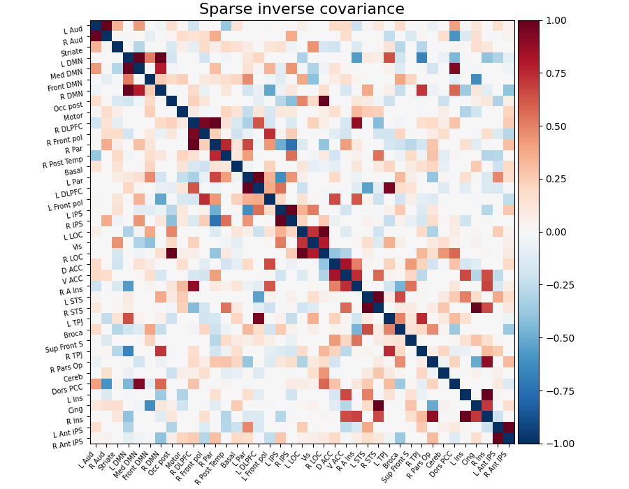
Note that the inverse covariance (or precision) contains values that can be linked to negated partial correlations, so we negated it for display.

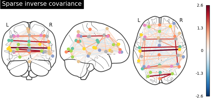
As the MSDL atlas comes with (x, y, z) MNI coordinates for the different regions, we can visualize the matrix as a graph of interaction in a brain. To avoid having too dense a graph, we represent only the 20% edges with the highest values.

Note

If you are using Nilearn with a version older than 0.9.0, then you should either upgrade your version or import maskers from the input_data module instead of the maskers module.

That is, you should manually replace in the following example all occurrences of:

from nilearn.maskers import NiftiMasker

with:

from nilearn.input_data import NiftiMasker

Retrieve the atlas and the data

from nilearn import datasets

atlas = datasets.fetch_atlas_msdl()
# Loading atlas image stored in 'maps'
atlas_filename = atlas["maps"]
# Loading atlas data stored in 'labels'
labels = atlas["labels"]

# Loading the functional datasets
data = datasets.fetch_development_fmri(n_subjects=1)

# print basic information on the dataset
print(f"First subject functional nifti images (4D) are at: {data.func[0]}")

First subject functional nifti images (4D) are at: /home/runner/work/nilearn/nilearn/nilearn_data/development_fmri/development_fmri/sub-pixar123_task-pixar_space-MNI152NLin2009cAsym_desc-preproc_bold.nii.gz

Extract time series

from nilearn.maskers import NiftiMapsMasker

masker = NiftiMapsMasker(
    maps_img=atlas_filename,
    standardize="zscore_sample",
    standardize_confounds="zscore_sample",
    memory="nilearn_cache",
    verbose=5,
)

time_series = masker.fit_transform(data.func[0], confounds=data.confounds)

[NiftiMapsMasker.wrapped] loading regions from None
Resampling maps
/opt/hostedtoolcache/Python/3.12.3/x64/lib/python3.12/site-packages/nilearn/maskers/base_masker.py:270: UserWarning:

memory_level is currently set to 0 but a Memory object has been provided. Setting memory_level to 1.

________________________________________________________________________________
[Memory] Calling nilearn.image.resampling.resample_img...
resample_img(<nibabel.nifti1.Nifti1Image object at 0x7f853d94db80>, interpolation='continuous', target_shape=(50, 59, 50), target_affine=array([[   4.,    0.,    0.,  -96.],
       [   0.,    4.,    0., -132.],
       [   0.,    0.,    4.,  -78.],
       [   0.,    0.,    0.,    1.]]))
_____________________________________________________resample_img - 1.2s, 0.0min
________________________________________________________________________________
[Memory] Calling nilearn.maskers.base_masker._filter_and_extract...
_filter_and_extract('/home/runner/work/nilearn/nilearn/nilearn_data/development_fmri/development_fmri/sub-pixar123_task-pixar_space-MNI152NLin2009cAsym_desc-preproc_bold.nii.gz',
<nilearn.maskers.nifti_maps_masker._ExtractionFunctor object at 0x7f853d94de20>, { 'allow_overlap': True,
  'clean_kwargs': {},
  'detrend': False,
  'dtype': None,
  'high_pass': None,
  'high_variance_confounds': False,
  'keep_masked_maps': True,
  'low_pass': None,
  'maps_img': '/home/runner/work/nilearn/nilearn/nilearn_data/msdl_atlas/MSDL_rois/msdl_rois.nii',
  'mask_img': None,
  'reports': True,
  'smoothing_fwhm': None,
  'standardize': 'zscore_sample',
  'standardize_confounds': 'zscore_sample',
  't_r': None,
  'target_affine': None,
  'target_shape': None}, confounds=[ '/home/runner/work/nilearn/nilearn/nilearn_data/development_fmri/development_fmri/sub-pixar123_task-pixar_desc-reducedConfounds_regressors.tsv'], sample_mask=None, dtype=None, memory=Memory(location=nilearn_cache/joblib), memory_level=1, verbose=5)
[NiftiMapsMasker.transform_single_imgs] Loading data from /home/runner/work/nilearn/nilearn/nilearn_data/development_fmri/development_fmri/sub-pixar123_task-pixar_space-MNI152NLin2009cAsym_desc-preproc_bold.nii.gz
[NiftiMapsMasker.transform_single_imgs] Extracting region signals
[NiftiMapsMasker.transform_single_imgs] Cleaning extracted signals
_______________________________________________filter_and_extract - 1.3s, 0.0min

Compute the sparse inverse covariance

try:
    from sklearn.covariance import GraphicalLassoCV
except ImportError:
    # for Scitkit-Learn < v0.20.0
    from sklearn.covariance import GraphLassoCV as GraphicalLassoCV

estimator = GraphicalLassoCV()
estimator.fit(time_series)

GraphicalLassoCV()

In a Jupyter environment, please rerun this cell to show the HTML representation or trust the notebook.
On GitHub, the HTML representation is unable to render, please try loading this page with nbviewer.org.

Display the connectome matrix

from nilearn import plotting

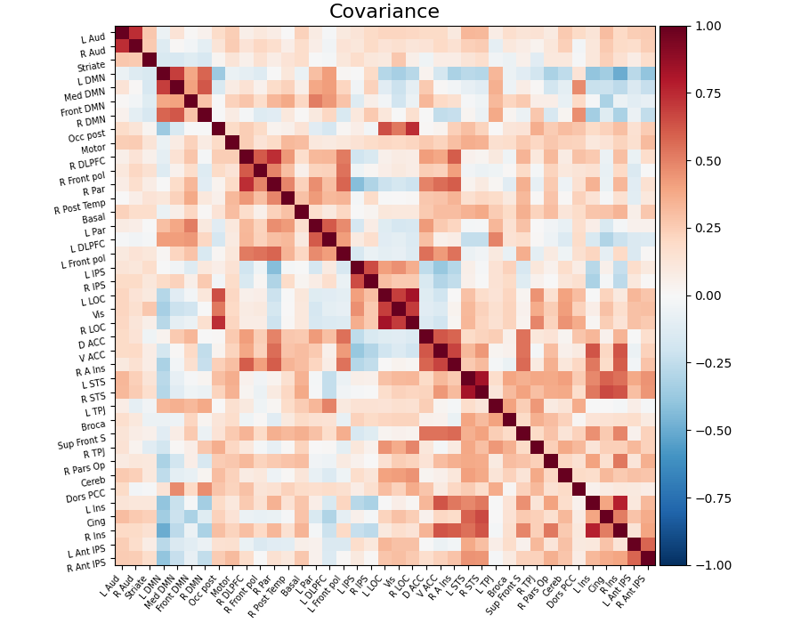
# Display the covariance

# The covariance can be found at estimator.covariance_
plotting.plot_matrix(
    estimator.covariance_,
    labels=labels,
    figure=(9, 7),
    vmax=1,
    vmin=-1,
    title="Covariance",
)

<matplotlib.image.AxesImage object at 0x7f853d94f4d0>

And now display the corresponding graph

coords = atlas.region_coords

plotting.plot_connectome(estimator.covariance_, coords, title="Covariance")

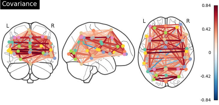
<nilearn.plotting.displays._projectors.OrthoProjector object at 0x7f853daa4920>

Display the sparse inverse covariance

we negate it to get partial correlations

plotting.plot_matrix(
    -estimator.precision_,
    labels=labels,
    figure=(9, 7),
    vmax=1,
    vmin=-1,
    title="Sparse inverse covariance",
)

<matplotlib.image.AxesImage object at 0x7f853d7fc980>

And now display the corresponding graph

plotting.plot_connectome(
    -estimator.precision_, coords, title="Sparse inverse covariance"
)

plotting.show()

3D visualization in a web browser

An alternative to nilearn.plotting.plot_connectome is to use nilearn.plotting.view_connectome that gives more interactive visualizations in a web browser. See 3D Plots of connectomes for more details.

view = plotting.view_connectome(-estimator.precision_, coords)

# In a Jupyter notebook, if ``view`` is the output of a cell, it will
# be displayed below the cell
view

# uncomment this to open the plot in a web browser:
# view.open_in_browser()

Estimated memory usage: 1333 MB