Voxel-Based Morphometry on OASIS dataset

This example uses voxel-based morphometry (VBM) to study the relationship between aging, sex, and gray matter density.

The data come from the OASIS project. If you use it, you need to agree with the data usage agreement available on the website.

It has been run through a standard VBM pipeline (using SPM8 and NewSegment) to create VBM maps, which we study here.

VBM analysis of aging

We run a standard GLM analysis to study the association between age and gray matter density from the VBM data. We use only 100 subjects from the OASIS dataset to limit the memory usage.

Note that more power would be obtained from using a larger sample of subjects.

Load Oasis dataset

from nilearn import datasets, plotting

n_subjects = 100  # more subjects requires more memory

oasis_dataset = datasets.fetch_oasis_vbm(
    n_subjects=n_subjects,
    legacy_format=False,
)
gray_matter_map_filenames = oasis_dataset.gray_matter_maps
age = oasis_dataset.ext_vars["age"].astype(float)

Sex is encoded as ‘M’ or ‘F’. Hence, we make it a binary variable.

sex = oasis_dataset.ext_vars["mf"] == "F"

Print basic information on the dataset.

print(
    "First gray-matter anatomy image (3D) is located at: "
    f"{oasis_dataset.gray_matter_maps[0]}"
)
print(
    "First white-matter anatomy image (3D) is located at: "
    f"{oasis_dataset.white_matter_maps[0]}"
)

First gray-matter anatomy image (3D) is located at: /home/runner/work/nilearn/nilearn/nilearn_data/oasis1/OAS1_0001_MR1/mwrc1OAS1_0001_MR1_mpr_anon_fslswapdim_bet.nii.gz
First white-matter anatomy image (3D) is located at: /home/runner/work/nilearn/nilearn/nilearn_data/oasis1/OAS1_0001_MR1/mwrc2OAS1_0001_MR1_mpr_anon_fslswapdim_bet.nii.gz

Get a mask image: A mask of the cortex of the ICBM template.

gm_mask = datasets.fetch_icbm152_brain_gm_mask()

Resample the mask, since this mask has a different resolution.

from nilearn.image import resample_to_img

mask_img = resample_to_img(
    gm_mask,
    gray_matter_map_filenames[0],
    interpolation="nearest",
)

Analyse data

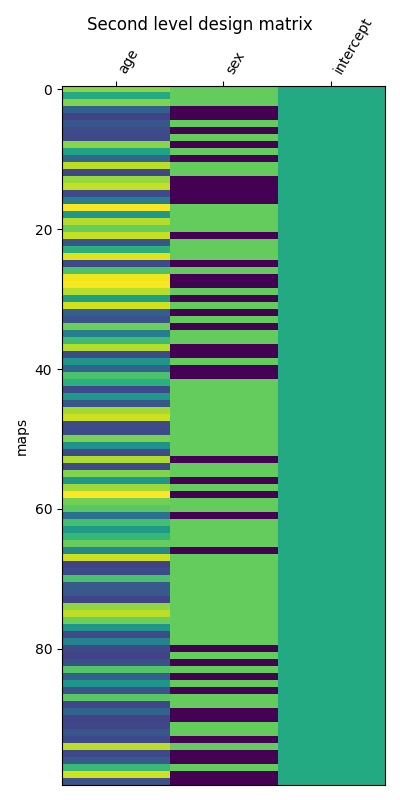
First, we create an adequate design matrix with three columns: ‘age’, ‘sex’, and ‘intercept’.

import numpy as np
import pandas as pd

intercept = np.ones(n_subjects)
design_matrix = pd.DataFrame(
    np.vstack((age, sex, intercept)).T,
    columns=["age", "sex", "intercept"],
)

from matplotlib import pyplot as plt

Let’s plot the design matrix.

fig, ax1 = plt.subplots(1, 1, figsize=(4, 8))
ax = plotting.plot_design_matrix(design_matrix, ax=ax1)
ax.set_ylabel("maps")
fig.suptitle("Second level design matrix")

Text(0.5, 0.98, 'Second level design matrix')

Next, we specify and fit the second-level model when loading the data and also smooth a little bit to improve statistical behavior.

from nilearn.glm.second_level import SecondLevelModel

second_level_model = SecondLevelModel(
    smoothing_fwhm=2.0, mask_img=mask_img, n_jobs=2, minimize_memory=False
)
second_level_model.fit(
    gray_matter_map_filenames,
    design_matrix=design_matrix,
)

SecondLevelModel(mask_img=<nibabel.nifti1.Nifti1Image object at 0x7f852ce80080>,
                 memory=Memory(location=None), minimize_memory=False, n_jobs=2,
                 smoothing_fwhm=2.0)

In a Jupyter environment, please rerun this cell to show the HTML representation or trust the notebook.
On GitHub, the HTML representation is unable to render, please try loading this page with nbviewer.org.

Estimating the contrast is very simple. We can just provide the column name of the design matrix.

z_map = second_level_model.compute_contrast(
    second_level_contrast=[1, 0, 0],
    output_type="z_score",
)

We threshold the second level contrast at FDR-corrected p < 0.05 and plot it.

from nilearn.glm import threshold_stats_img

_, threshold = threshold_stats_img(z_map, alpha=0.05, height_control="fdr")
print(f"The FDR=.05-corrected threshold is: {threshold:03g}")

fig = plt.figure(figsize=(5, 3))
display = plotting.plot_stat_map(
    z_map,
    threshold=threshold,
    colorbar=True,
    display_mode="z",
    cut_coords=[-4, 26],
    figure=fig,
)
fig.suptitle("age effect on gray matter density (FDR = .05)")
plotting.show()

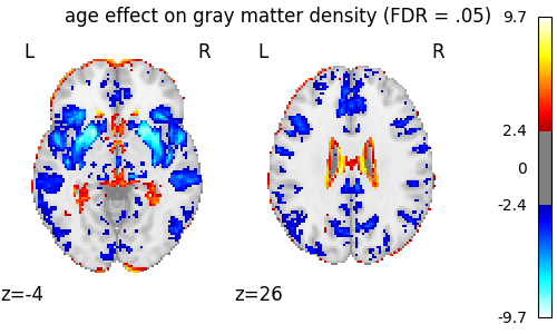
The FDR=.05-corrected threshold is: 2.40175

We can also study the effect of sex by computing the contrast, thresholding it and plot the resulting map.

z_map = second_level_model.compute_contrast(
    second_level_contrast="sex",
    output_type="z_score",
)
_, threshold = threshold_stats_img(z_map, alpha=0.05, height_control="fdr")
plotting.plot_stat_map(
    z_map,
    threshold=threshold,
    colorbar=True,
    title="sex effect on gray matter density (FDR = .05)",
)

<nilearn.plotting.displays._slicers.OrthoSlicer object at 0x7f852ce82780>

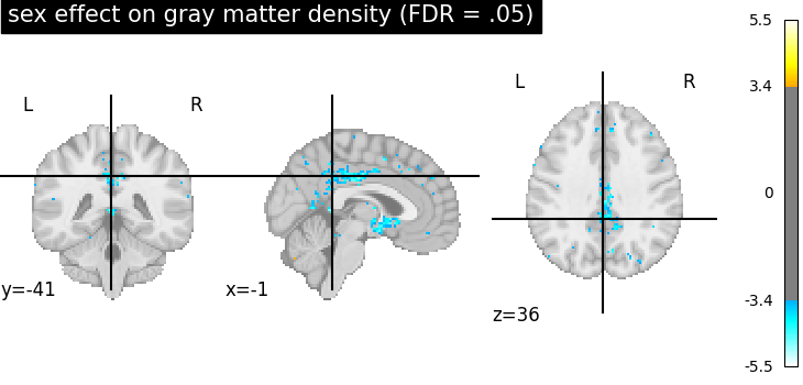
Note that there does not seem to be any significant effect of sex on gray matter density on that dataset.

Generating a report

It can be useful to quickly generate a portable, ready-to-view report with most of the pertinent information. This is easy to do if you have a fitted model and the list of contrasts, which we do here.

from nilearn.reporting import make_glm_report

icbm152_2009 = datasets.fetch_icbm152_2009()
report = make_glm_report(
    model=second_level_model,
    contrasts=["age", "sex"],
    bg_img=icbm152_2009["t1"],
)

We have several ways to access the report: report # This report can be viewed in a notebook report.open_in_browser()

# or we can save as an html file
from pathlib import Path

output_dir = Path.cwd() / "results" / "plot_oasis"
output_dir.mkdir(exist_ok=True, parents=True)
report.save_as_html(output_dir / "report.html")

Saving model outputs to disk

# We can also save the model outputs to disk
from nilearn.interfaces.bids import save_glm_to_bids

save_glm_to_bids(
    second_level_model,
    contrasts=["age", "sex"],
    out_dir=output_dir / "derivatives" / "nilearn_glm",
    prefix="ageEffectOnGM",
    bg_img=icbm152_2009["t1"],
)

• 
• 
• 

View the generated files

files = sorted(list((output_dir / "derivatives" / "nilearn_glm").glob("**/*")))
print("\n".join([str(x.relative_to(output_dir)) for x in files]))

derivatives/nilearn_glm/dataset_description.json
derivatives/nilearn_glm/group
derivatives/nilearn_glm/group/ageEffectOnGM_contrast-age_design.svg
derivatives/nilearn_glm/group/ageEffectOnGM_contrast-age_stat-effect_statmap.nii.gz
derivatives/nilearn_glm/group/ageEffectOnGM_contrast-age_stat-p_statmap.nii.gz
derivatives/nilearn_glm/group/ageEffectOnGM_contrast-age_stat-t_statmap.nii.gz
derivatives/nilearn_glm/group/ageEffectOnGM_contrast-age_stat-variance_statmap.nii.gz
derivatives/nilearn_glm/group/ageEffectOnGM_contrast-age_stat-z_statmap.nii.gz
derivatives/nilearn_glm/group/ageEffectOnGM_contrast-sex_design.svg
derivatives/nilearn_glm/group/ageEffectOnGM_contrast-sex_stat-effect_statmap.nii.gz
derivatives/nilearn_glm/group/ageEffectOnGM_contrast-sex_stat-p_statmap.nii.gz
derivatives/nilearn_glm/group/ageEffectOnGM_contrast-sex_stat-t_statmap.nii.gz
derivatives/nilearn_glm/group/ageEffectOnGM_contrast-sex_stat-variance_statmap.nii.gz
derivatives/nilearn_glm/group/ageEffectOnGM_contrast-sex_stat-z_statmap.nii.gz
derivatives/nilearn_glm/group/ageEffectOnGM_design.svg
derivatives/nilearn_glm/group/ageEffectOnGM_design.tsv
derivatives/nilearn_glm/group/ageEffectOnGM_report.html
derivatives/nilearn_glm/group/ageEffectOnGM_stat-errorts_statmap.nii.gz
derivatives/nilearn_glm/group/ageEffectOnGM_stat-rsquared_statmap.nii.gz
derivatives/nilearn_glm/group/ageEffectOnGM_statmap.json

Estimated memory usage: 2616 MB