Deriving spatial maps from group fMRI data using ICA and Dictionary Learning

Various approaches exist to derive spatial maps or networks from group fMRI data. The methods extract distributed brain regions that exhibit similar BOLD fluctuations over time. Decomposition methods allow for generation of many independent maps simultaneously without the need to provide a priori information (e.g. seeds or priors).

This example will apply two popular decomposition methods, ICA and Dictionary learning, to fMRI data measured while children and young adults watch movies. The resulting maps will be visualized using atlas plotting tools.

CanICA is an ICA method for group-level analysis of fMRI data. Compared to other strategies, it brings a well-controlled group model, as well as a thresholding algorithm controlling for specificity and sensitivity with an explicit model of the signal.

The reference paper is Varoquaux et al.[1].

Load brain development fMRI dataset

from nilearn.datasets import fetch_development_fmri

rest_dataset = fetch_development_fmri(n_subjects=30)
func_filenames = rest_dataset.func  # list of 4D nifti files for each subject

# print basic information on the dataset
print(f"First functional nifti image (4D) is at: {rest_dataset.func[0]}")

[fetch_development_fmri] Dataset directory found: /home/runner/work/nilearn/nilearn/nilearn_data/development_fmri
First functional nifti image (4D) is at: /home/runner/work/nilearn/nilearn/nilearn_data/development_fmri/sub-pixar128_task-pixar_space-MNI152NLin2009cAsym_desc-preproc_bold.nii.gz

Apply CanICA on the data

We use “whole-brain-template” as a strategy to compute the mask, as this leads to slightly faster and more reproducible results. However, the images need to be in MNI template space.

import warnings

from sklearn.exceptions import ConvergenceWarning

from nilearn.decomposition import CanICA

canica = CanICA(
    n_components=20,
    memory="nilearn_cache",
    memory_level=1,
    verbose=1,
    random_state=0,
    mask_strategy="whole-brain-template",
    n_jobs=2,
)
with warnings.catch_warnings():
    # silence warnings about ICA not converging
    # Consider increasing tolerance or the maximum number of iterations.
    warnings.filterwarnings(action="ignore", category=ConvergenceWarning)
    canica.fit(func_filenames)

[CanICA.fit] Loading data
[Parallel(n_jobs=2)]: Using backend LokyBackend with 2 concurrent workers.
[Parallel(n_jobs=2)]: Done  10 out of  10 | elapsed:   15.2s finished

Visualize the results

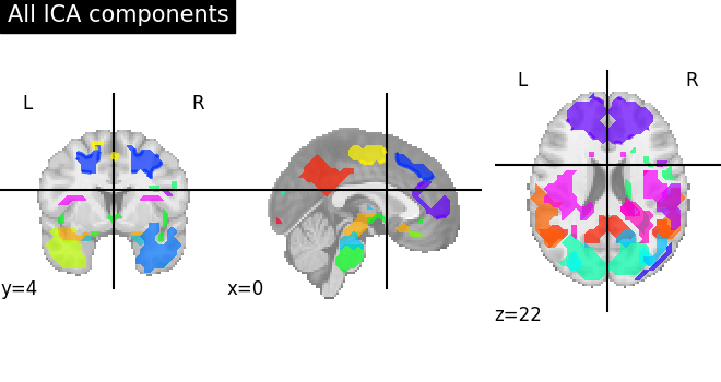
To visualize, we retrieve the independent components in brain space directly accessible through attribute components_img_. We then plot the outline of all ICA components on one figure.

from nilearn.plotting import plot_prob_atlas

canica_components_img = canica.components_img_

plot_prob_atlas(canica_components_img, title="All ICA components")

/home/runner/work/nilearn/nilearn/.tox/doc/lib/python3.11/site-packages/numpy/ma/core.py:2820: UserWarning:

Warning: converting a masked element to nan.


<nilearn.plotting.displays._slicers.OrthoSlicer object at 0x7f17b6afa990>

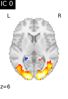
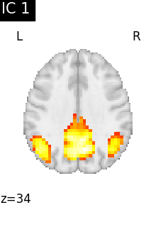
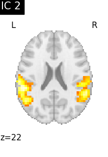
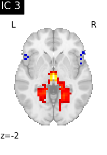
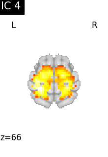
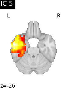
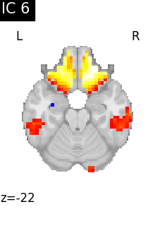
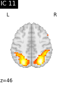
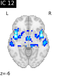
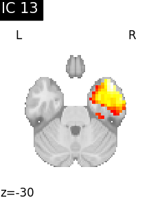
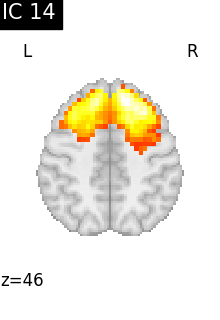
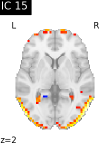
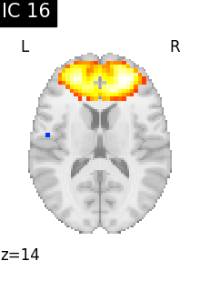
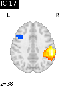
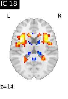
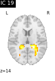
Finally, we plot the map for each ICA component separately.

Note

The following code block will generate many figures.

from nilearn.image import iter_img
from nilearn.plotting import plot_stat_map, show

for i, cur_img in enumerate(iter_img(canica_components_img)):
    plot_stat_map(
        cur_img,
        display_mode="z",
        title=f"IC {int(i)}",
        cut_coords=1,
        vmax=0.05,
        vmin=-0.05,
        colorbar=False,
    )

show()

• 
• 
• 
• 
• 
• 
• 
• 
• 
• 
• 
• 
• 
• 
• 
• 
• 
• 
• 
• 

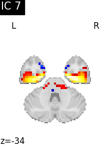
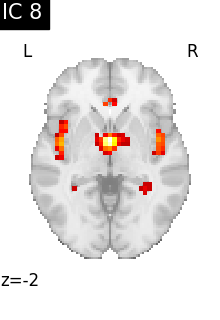
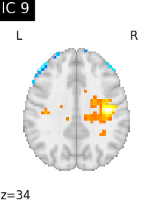
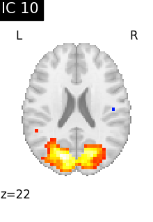
Compare CanICA to dictionary learning

Dictionary learning is a sparsity based decomposition method for extracting spatial maps. It extracts maps that are naturally sparse and usually cleaner than ICA. Here, we will compare networks built with CanICA to networks built with Dictionary learning.

For more details see Mensch et al.[2].

Create a dictionary learning estimator

from nilearn.decomposition import DictLearning

dict_learning = DictLearning(
    n_components=20,
    memory="nilearn_cache",
    memory_level=1,
    verbose=1,
    random_state=0,
    n_epochs=1,
    mask_strategy="whole-brain-template",
    n_jobs=2,
)

dict_learning.fit(func_filenames)

[DictLearning.fit] Loading data
[DictLearning.fit] Learning initial components
[Parallel(n_jobs=2)]: Using backend LokyBackend with 2 concurrent workers.
[DictLearning.fit] Computing initial loadings
________________________________________________________________________________
[Memory] Calling nilearn.decomposition.dict_learning._compute_loadings...
_compute_loadings(array([[ 0.007659, ...,  0.006189],
       ...,
       [-0.001064, ...,  0.00268 ]]),
array([[-0.280625, ...,  0.825802],
       ...,
       [-0.997198, ..., -0.015035]]))
_________________________________________________compute_loadings - 0.0s, 0.0min
[DictLearning.fit]  Learning dictionary
________________________________________________________________________________
[Memory] Calling sklearn.decomposition._dict_learning.dict_learning_online...
dict_learning_online(array([[-0.280625, ..., -0.997198],
       ...,
       [ 0.825802, ..., -0.015035]]),
20, alpha=10, batch_size=20, method='cd', dict_init=array([[-0.107744, ..., -0.01632 ],
       ...,
       [ 0.349894, ..., -0.191299]]), verbose=0, random_state=0, return_code=True, shuffle=True, n_jobs=1, max_iter=1090)
_____________________________________________dict_learning_online - 2.4s, 0.0min

DictLearning(mask_strategy='whole-brain-template', memory='nilearn_cache',
             memory_level=1, n_jobs=2, random_state=0, verbose=1)

In a Jupyter environment, please rerun this cell to show the HTML representation or trust the notebook.
On GitHub, the HTML representation is unable to render, please try loading this page with nbviewer.org.

Visualize the results

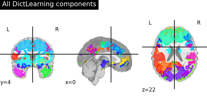
First plot all DictLearning components together

dictlearning_components_img = dict_learning.components_img_
plot_prob_atlas(
    dictlearning_components_img, title="All DictLearning components"
)

/home/runner/work/nilearn/nilearn/.tox/doc/lib/python3.11/site-packages/numpy/ma/core.py:2820: UserWarning:

Warning: converting a masked element to nan.


<nilearn.plotting.displays._slicers.OrthoSlicer object at 0x7f17ba7b34d0>

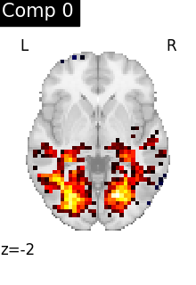
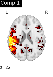
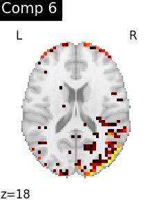
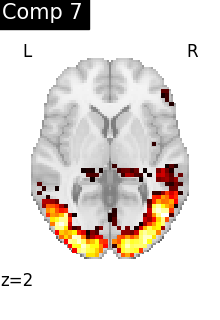
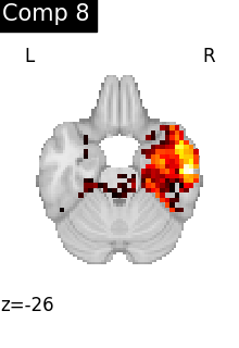
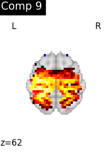
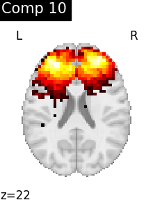
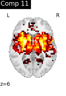
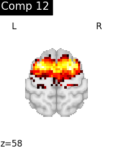
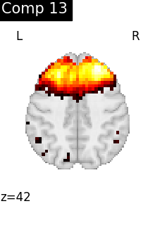
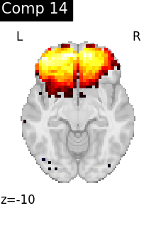
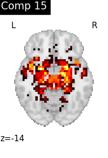
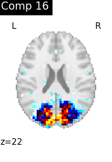
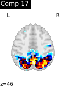
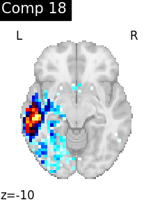
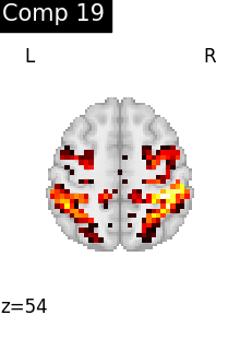
One plot of each component

Note

The following code block will generate many figures.

for i, cur_img in enumerate(iter_img(dictlearning_components_img)):
    plot_stat_map(
        cur_img,
        display_mode="z",
        title=f"Comp {int(i)}",
        cut_coords=1,
        vmax=0.1,
        vmin=-0.1,
        colorbar=False,
    )

• 
• 
• 
• 
• 
• 
• 
• 
• 
• 
• 
• 
• 
• 
• 
• 
• 
• 
• 
• 

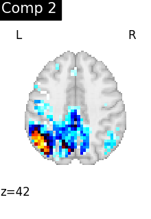
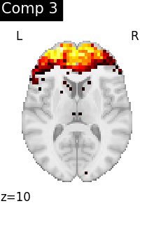
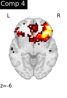
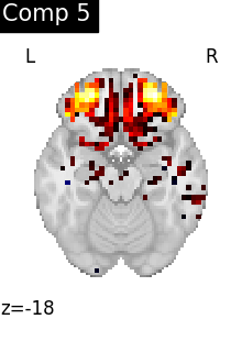
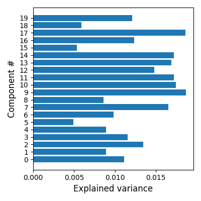
Estimate explained variance per component and plot using matplotlib.

The fitted object dict_learning can be used to calculate the score per component.

scores = dict_learning.score(func_filenames, per_component=True)

________________________________________________________________________________
[Memory] Calling nilearn.decomposition._base._explained_variance...
_explained_variance(array([[-2.806378e-01, ...,  8.257976e-01],
       ...,
       [-2.017024e-15, ..., -6.232236e-16]]),
array([[0., ..., 0.],
       ...,
       [0., ..., 0.]]), per_component=True)
______________________________________________explained_variance - 16.6s, 0.3min

Plot the scores

import numpy as np
from matplotlib import pyplot as plt
from matplotlib.ticker import FormatStrFormatter

plt.figure(figsize=(4, 4), constrained_layout=True)

positions = np.arange(len(scores))
plt.barh(positions, scores)
plt.ylabel("Component #", size=12)
plt.xlabel("Explained variance", size=12)
plt.yticks(np.arange(20))
plt.gca().xaxis.set_major_formatter(FormatStrFormatter("%.3f"))

show()

Note

To see how to extract subject-level timeseries from regions created using Dictionary learning, see example Regions extraction using dictionary learning and functional connectomes.

References

[1]

Gael Varoquaux, Sepideh Sadaghiani, Philippe Pinel, Andreas Kleinschmidt, Jean-Baptiste Poline, and Bertrand Thirion. A group model for stable multi-subject ica on fmri datasets. NeuroImage, 51(1):288–299, 2010. URL: https://pubmed.ncbi.nlm.nih.gov/20153834, doi:10.1016/j.neuroimage.2010.02.010.

[2]

Arthur Mensch, Gael Varoquaux, and Bertrand Thirion. Compressed online dictionary learning for fast resting-state fmri decomposition. In 2016 IEEE 13th International Symposium on Biomedical Imaging (ISBI), volume, 1282–1285. 2016. doi:10.1109/ISBI.2016.7493501.

Estimated memory usage: 2733 MB