NeuroVault meta-analysis of stop-go paradigm studies

This example shows how to download statistical maps from Neurovault.

See fetch_neurovault_ids documentation for more details.

import scipy

from nilearn import plotting
from nilearn.datasets import fetch_neurovault_ids
from nilearn.image import get_data, load_img, math_img, new_img_like

Fetch images for “successful stop minus go”-like protocols.

# These are the images we are interested in,
# in order to save time we specify their ids explicitly.
stop_go_image_ids = (151, 3041, 3042, 2676, 2675, 2818, 2834)

# These ids were determined by querying Neurovault like this:

# from nilearn.datasets import fetch_neurovault, neurovault
#
# nv_data = fetch_neurovault(
#     max_images=7,
#     cognitive_paradigm_cogatlas=neurovault.Contains('stop signal'),
#     contrast_definition=neurovault.Contains('succ', 'stop', 'go'),
#     map_type='T map')
#
# print([meta['id'] for meta in nv_data['images_meta']])

nv_data = fetch_neurovault_ids(image_ids=stop_go_image_ids)

images_meta = nv_data["images_meta"]

[get_dataset_dir] Dataset found in /home/runner/nilearn_data/neurovault
[fetch_neurovault_ids] Reading local neurovault data.
[fetch_neurovault_ids] No image found on local disk.
[fetch_neurovault_ids] getting new batch: https://neurovault.org/api/images/3041
[_fetch_neurovault_implementation] getting new batch:
https://neurovault.org/api/collections/42
[fetch_neurovault_ids] Downloading file:
http://neurovault.org/media/images/42/task002_cope10_succstop_minus_go.nii.gz
[fetch_neurovault_ids] Download succeeded, downloaded to:
/home/runner/nilearn_data/neurovault/collection_42/image_3041.nii.gz
[fetch_neurovault_ids] Already fetched 1 image
[fetch_neurovault_ids] getting new batch: https://neurovault.org/api/images/3042
[_fetch_neurovault_implementation] getting new batch:
https://neurovault.org/api/collections/98
[fetch_neurovault_ids] Downloading file:
http://neurovault.org/media/images/98/task002_cope06_succ_stop_vs_go.nii.gz
[fetch_neurovault_ids] Download succeeded, downloaded to:
/home/runner/nilearn_data/neurovault/collection_98/image_3042.nii.gz
[fetch_neurovault_ids] Already fetched 2 images
[fetch_neurovault_ids] getting new batch: https://neurovault.org/api/images/2818
[_fetch_neurovault_implementation] getting new batch:
https://neurovault.org/api/collections/423
[fetch_neurovault_ids] Downloading file:
http://neurovault.org/media/images/423/task002_cope007_tstat1.nii.gz
[fetch_neurovault_ids] Download succeeded, downloaded to:
/home/runner/nilearn_data/neurovault/collection_423/image_2818.nii.gz
[fetch_neurovault_ids] Already fetched 3 images
[fetch_neurovault_ids] getting new batch: https://neurovault.org/api/images/2834
[fetch_neurovault_ids] Downloading file:
http://neurovault.org/media/images/423/task003_cope007_tstat1.nii.gz
[fetch_neurovault_ids] Download succeeded, downloaded to:
/home/runner/nilearn_data/neurovault/collection_423/image_2834.nii.gz
[fetch_neurovault_ids] Already fetched 4 images
[fetch_neurovault_ids] getting new batch: https://neurovault.org/api/images/2675
[_fetch_neurovault_implementation] getting new batch:
https://neurovault.org/api/collections/413
[fetch_neurovault_ids] Downloading file:
http://neurovault.org/media/images/413/A_model001_task002_cope011_tstat1.nii.gz
[fetch_neurovault_ids] Download succeeded, downloaded to:
/home/runner/nilearn_data/neurovault/collection_413/image_2675.nii.gz
[fetch_neurovault_ids] Already fetched 5 images
[fetch_neurovault_ids] getting new batch: https://neurovault.org/api/images/2676
[fetch_neurovault_ids] Downloading file:
http://neurovault.org/media/images/413/B_model001_task002_cope011_tstat1.nii.gz
[fetch_neurovault_ids] Download succeeded, downloaded to:
/home/runner/nilearn_data/neurovault/collection_413/image_2676.nii.gz
[fetch_neurovault_ids] Already fetched 6 images
[fetch_neurovault_ids] getting new batch: https://neurovault.org/api/images/151
[fetch_neurovault_ids] Downloading file:
http://neurovault.org/media/images/42/task001_cope07_succstop_minus_go.nii.gz
[fetch_neurovault_ids] Download succeeded, downloaded to:
/home/runner/nilearn_data/neurovault/collection_42/image_151.nii.gz
[fetch_neurovault_ids] Already fetched 7 images

Visualize the data

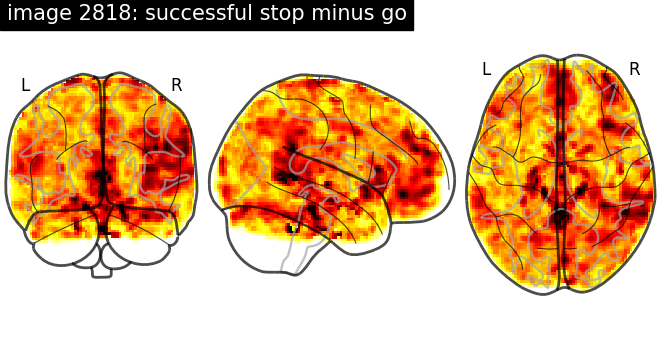
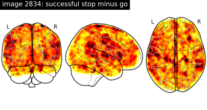
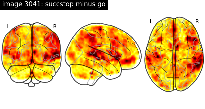
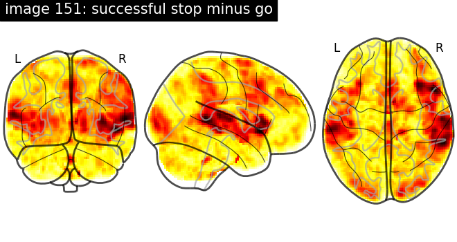
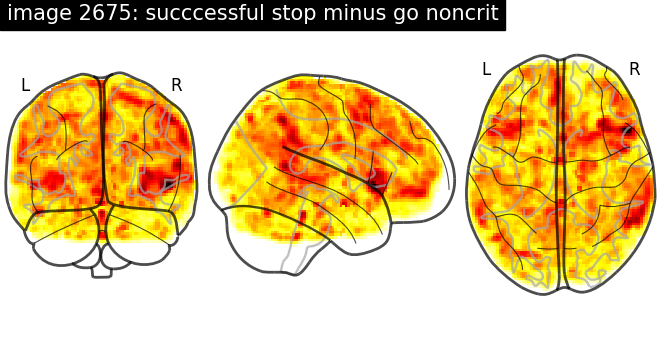
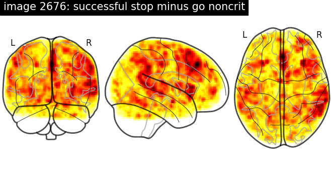
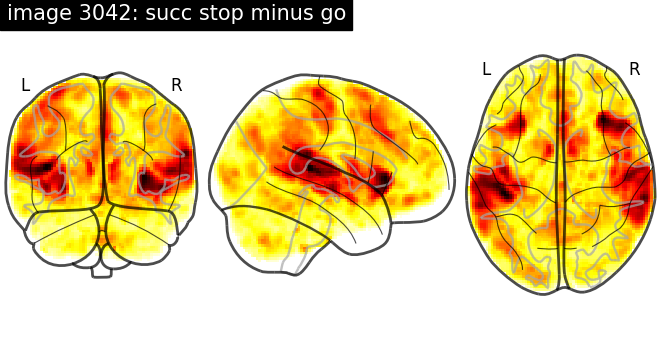
print("\nplotting glass brain for collected images\n")

for im in images_meta:
    plotting.plot_glass_brain(
        im["absolute_path"],
        title=f"image {im['id']}: {im['contrast_definition']}",
    )

• 
• 
• 
• 
• 
• 
• 

plotting glass brain for collected images

Compute statistics

def t_to_z(t_scores, deg_of_freedom):
    """Convert t-scores to z-scores."""
    p_values = scipy.stats.t.sf(t_scores, df=deg_of_freedom)
    z_values = scipy.stats.norm.isf(p_values)
    return z_values


# Compute z values
z_imgs = []
current_collection = None

print("\nComputing maps...")

# convert t to z for all images
for this_meta in images_meta:
    if this_meta["collection_id"] != current_collection:
        print(f"\n\nCollection {this_meta['id']}:")
        current_collection = this_meta["collection_id"]

    # Load and validate the downloaded image.
    t_img = load_img(this_meta["absolute_path"])
    deg_of_freedom = this_meta["number_of_subjects"] - 2
    print(
        f"     Image {this_meta['id']}: degrees of freedom: {deg_of_freedom}"
    )

    # Convert data, create new image.
    z_img = new_img_like(
        t_img, t_to_z(get_data(t_img), deg_of_freedom=deg_of_freedom)
    )

    z_imgs.append(z_img)

Computing maps...


Collection 3041:
     Image 3041: degrees of freedom: 13


Collection 3042:
     Image 3042: degrees of freedom: 22


Collection 2818:
     Image 2818: degrees of freedom: 18
     Image 2834: degrees of freedom: 18


Collection 2675:
     Image 2675: degrees of freedom: 6
     Image 2676: degrees of freedom: 6


Collection 151:
     Image 151: degrees of freedom: 13

Plot the combined z maps

cut_coords = [-15, -8, 6, 30, 46, 62]
meta_analysis_img = math_img(
    "np.sum(z_imgs, axis=3) / np.sqrt(z_imgs.shape[3])", z_imgs=z_imgs
)

plotting.plot_stat_map(
    meta_analysis_img,
    display_mode="z",
    threshold=6,
    cut_coords=cut_coords,
    vmax=12,
)

plotting.show()

Estimated memory usage: 160 MB