Classification of age groups using functional connectivity

This example compares different kinds of functional connectivity between regions of interest : correlation, partial correlation, and tangent space embedding.

The resulting connectivity coefficients can be used to discriminate children from adults. In general, the tangent space embedding outperforms the standard correlations: see Dadi et al.[1] for a careful study.

# overall verbosity of the example
verbose = 0

Load brain development fMRI dataset and MSDL atlas

We study only 30 subjects from the dataset, to save computation time.

from nilearn.datasets import fetch_atlas_msdl, fetch_development_fmri
from nilearn.plotting import (
    plot_connectome,
    plot_matrix,
    show,
)

development_dataset = fetch_development_fmri(n_subjects=30, verbose=verbose)

We use probabilistic regions of interest (ROIs) from the MSDL atlas.

msdl_data = fetch_atlas_msdl()
msdl_coords = msdl_data.region_coords
n_regions = len(msdl_coords)

print(
    f"MSDL has {n_regions} ROIs, "
    f"part of the following networks:\n{msdl_data.networks}."
)

[fetch_atlas_msdl] Dataset directory found: /home/runner/work/nilearn/nilearn/nilearn_data/msdl_atlas
MSDL has 39 ROIs, part of the following networks:
['Aud', 'Aud', 'Striate', 'DMN', 'DMN', 'DMN', 'DMN', 'Occ post', 'Motor', 'R V Att', 'R V Att', 'R V Att', 'R V Att', 'Basal', 'L V Att', 'L V Att', 'L V Att', 'D Att', 'D Att', 'Vis Sec', 'Vis Sec', 'Vis Sec', 'Salience', 'Salience', 'Salience', 'Temporal', 'Temporal', 'Language', 'Language', 'Language', 'Language', 'Language', 'Cereb', 'Dors PCC', 'Cing-Ins', 'Cing-Ins', 'Cing-Ins', 'Ant IPS', 'Ant IPS'].

Region signals extraction

To extract regions time series, we instantiate a MultiNiftiMapsMasker object and pass the atlas the file name to it, as well as filtering band-width and detrending option.

Then we compute region signals and extract useful phenotypic information, for all subjects and then group the outputs for children and adults.

from nilearn.maskers import MultiNiftiMapsMasker

masker = MultiNiftiMapsMasker(
    msdl_data.maps,
    resampling_target="data",
    t_r=development_dataset.t_r,
    detrend=True,
    low_pass=0.1,
    high_pass=0.01,
    standardize="zscore_sample",
    memory="nilearn_cache",
    memory_level=1,
    standardize_confounds=True,
    verbose=verbose,
)

pooled_subjects = masker.fit_transform(
    development_dataset.func, confounds=development_dataset.confounds
)

groups = development_dataset.phenotypic["Child_Adult"].tolist()

children = []
for time_series, phenotype in zip(pooled_subjects, groups, strict=False):
    if phenotype == "child":
        children.append(time_series)

#  %%
print(f"Data has {len(children)} children.")

Data has 24 children.

ROI-to-ROI correlations of children

The simpler and most commonly used kind of connectivity is correlation. It models the full (marginal) connectivity between pairwise ROIs. We can estimate it using ConnectivityMeasure.

from nilearn.connectome import ConnectivityMeasure

correlation_measure = ConnectivityMeasure(kind="correlation", verbose=verbose)

From the list of ROIs time-series for children, the correlation_measure computes individual correlation matrices.

correlation_matrices = correlation_measure.fit_transform(children)

All individual coefficients are stacked in a unique 2D matrix. as well as the average correlation across all fitted subjects.

print(
    "Correlations of children are stacked "
    f"in an array of shape {correlation_matrices.shape}"
)

mean_correlation_matrix = correlation_measure.mean_
print(f"Mean correlation has shape {mean_correlation_matrix.shape}.")

Correlations of children are stacked in an array of shape (24, 39, 39)
Mean correlation has shape (39, 39).

We display the connectome matrices of the first 3 children.

import numpy as np
from matplotlib import pyplot as plt

_, axes = plt.subplots(1, 3, figsize=(15, 5))
vmax = np.absolute(correlation_matrices).max()
for i, (matrix, ax) in enumerate(
    zip(correlation_matrices, axes, strict=False)
):
    plot_matrix(
        matrix,
        tri="lower",
        axes=ax,
        title=f"correlation, child {i}",
        vmax=vmax,
        vmin=-vmax,
    )

show()

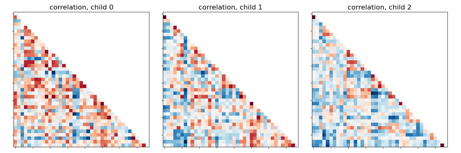
The blocks structure that reflect functional networks are visible.

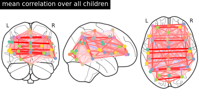
Now we display as a connectome the mean correlation matrix over all children.

plot_connectome(
    mean_correlation_matrix,
    msdl_coords,
    title="mean correlation over all children",
)

show()

Studying partial correlations

We can also study direct connections, revealed by partial correlation coefficients. We just change the ConnectivityMeasure kind.

partial_correlation_measure = ConnectivityMeasure(
    kind="partial correlation", verbose=verbose
)
partial_correlation_matrices = partial_correlation_measure.fit_transform(
    children
)

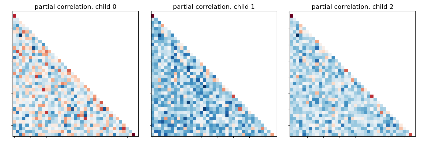
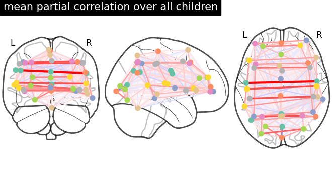
Most of direct connections are weaker than full connections.

_, axes = plt.subplots(1, 3, figsize=(15, 5))
vmax = np.absolute(partial_correlation_matrices).max()
for i, (matrix, ax) in enumerate(
    zip(partial_correlation_matrices, axes, strict=False)
):
    plot_matrix(
        matrix,
        tri="lower",
        axes=ax,
        title=f"partial correlation, child {i}",
        vmax=vmax,
        vmin=-vmax,
    )

plot_connectome(
    partial_correlation_measure.mean_,
    msdl_coords,
    title="mean partial correlation over all children",
)

show()

• 
• 

Extract subjects variabilities around a group connectivity

We can use both correlations and partial correlations to capture reproducible connectivity patterns at the group-level. This is done by the "tangent" space embedding.

tangent_measure = ConnectivityMeasure(kind="tangent", verbose=verbose)

We fit our children group to estimate the group connectivity matrix (stored in tangent_measure.mean_), and individual deviation matrices of each subject from it.

tangent_matrices = tangent_measure.fit_transform(children)

tangent_matrices model individual connectivities as perturbations of the group connectivity matrix tangent_measure.mean_. Keep in mind that these subjects-to-group variability matrices do not directly reflect individual brain connections. For instance negative coefficients cannot be interpreted as anticorrelated regions.

_, axes = plt.subplots(1, 3, figsize=(15, 5))
for i, (matrix, ax) in enumerate(zip(tangent_matrices, axes, strict=False)):
    plot_matrix(
        matrix,
        tri="lower",
        axes=ax,
        title=f"tangent offset, child {i}",
    )

show()

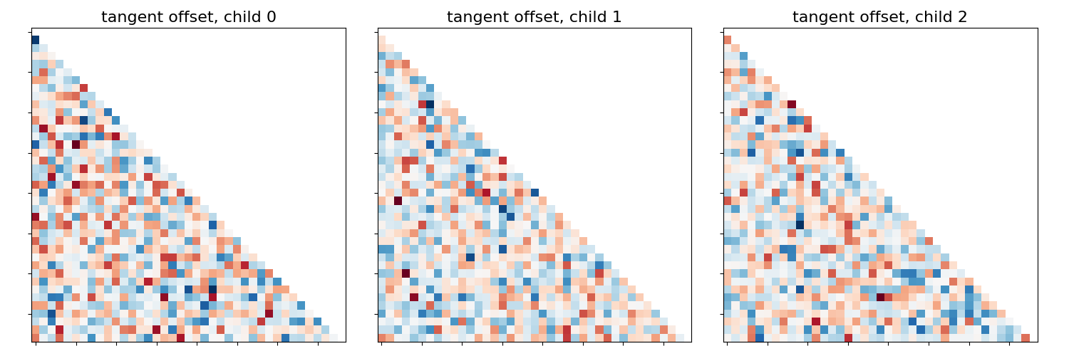
The average tangent matrix cannot be interpreted, as individual matrices represent deviations from the mean, which is set to 0.

What kind of connectivity is most powerful for classification?

We will use connectivity matrices as features to distinguish children from adults. We use cross-validation and measure classification accuracy to compare the different kinds of connectivity matrices. We use random splits of the subjects into training/testing sets. sklearn.model_selection.StratifiedShuffleSplit allows preserving the proportion of children in the test set. We also use sklearn.dummy.DummyClassifier to get the chance level performance. As the the proportion of children in the training/testing sets are preserved across all folds, we only need to calculate it once.

from sklearn.dummy import DummyClassifier
from sklearn.metrics import accuracy_score
from sklearn.model_selection import StratifiedShuffleSplit
from sklearn.svm import LinearSVC

kinds = ["correlation", "partial correlation", "tangent"]
_, classes = np.unique(groups, return_inverse=True)
cv = StratifiedShuffleSplit(n_splits=15, random_state=0, test_size=5)
pooled_subjects = np.asarray(pooled_subjects)

scores = {}
for kind in kinds:
    scores[kind] = []
    for train, test in cv.split(pooled_subjects, classes):
        # *ConnectivityMeasure* can output the estimated subjects coefficients
        # as a 1D arrays through the parameter *vectorize*.
        connectivity = ConnectivityMeasure(
            kind=kind, vectorize=True, verbose=verbose
        )
        # build vectorized connectomes for subjects in the train set
        connectomes = connectivity.fit_transform(pooled_subjects[train])
        # fit the classifier
        classifier = LinearSVC(dual=True, random_state=0, verbose=verbose).fit(
            connectomes, classes[train]
        )
        # make predictions for the left-out test subjects
        predictions = classifier.predict(
            connectivity.transform(pooled_subjects[test])
        )
        # store the accuracy for this cross-validation fold
        scores[kind].append(accuracy_score(classes[test], predictions))

        if not scores.get("dummy"):
            # run dummy classifier to get chance level performance
            # if its not there already
            dummy_prediction = (
                DummyClassifier()
                .fit(connectomes, classes[train])
                .predict(pooled_subjects[test])
            )
            scores["dummy"] = accuracy_score(classes[test], dummy_prediction)

display the results

mean_scores = [np.mean(scores[kind]) for kind in kinds]
scores_std = [np.std(scores[kind]) for kind in kinds]

plt.figure(figsize=(6, 4), constrained_layout=True)

positions = np.arange(len(kinds)) * 0.1 + 0.1
plt.barh(positions, mean_scores, align="center", height=0.05, xerr=scores_std)
yticks = [k.replace(" ", "\n") for k in kinds]
plt.yticks(positions, yticks)
plt.gca().grid(True)
plt.gca().set_axisbelow(True)
plt.gca().axvline(scores["dummy"], color="red", linestyle="--")
plt.xlabel("Classification accuracy\n(red line = chance level)")

show()

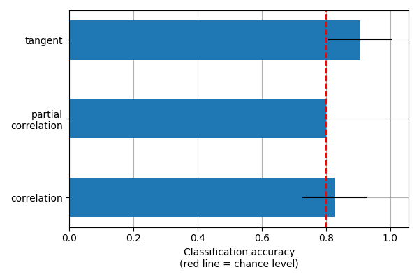
This is a small example to showcase nilearn features. In practice such comparisons need to be performed on much larger cohorts and several datasets. Dadi et al.[1] showed that across many cohorts and clinical questions, the tangent kind should be preferred.

References

[1] (1,2)

Kamalaker Dadi, Mehdi Rahim, Alexandre Abraham, Darya Chyzhyk, Michael Milham, Bertrand Thirion, and Gaël Varoquaux. Benchmarking functional connectome-based predictive models for resting-state fmri. NeuroImage, 192:115–134, 2019. doi:10.1016/j.neuroimage.2019.02.062.

Estimated memory usage: 6420 MB