Independent Component Analysis (ICA) of fMRI timeseries

This example applies the scikit-learn FastICA algorithm to fMRI data from a movie-watching task, accessed via the fetch_development_fmri fetcher.

Note that any unsupervised decomposition model — or other latent-factor models — can be accessed from scikit-learn and applied to the data by following the same procedure described in this example.

For decomposition methods that are specifically tailored to fMRI data, please refer to Deriving spatial maps from group fMRI data using ICA and Dictionary Learning.

Load the movie-watching dataset

Here we use only single subject fMRI timeseries for computational efficiency. We quickly check the size of this timeseries.

from nilearn import datasets, image

dataset = datasets.fetch_development_fmri(n_subjects=1)
func_filename = dataset.func[0]

# Print basic information on the dataset.
img = image.load_img(dataset.func[0])
print(f"Functional nifti image (4D) is of shape: {img.shape}")

[fetch_development_fmri] Dataset directory found: /home/runner/work/nilearn/nilearn/nilearn_data/development_fmri
Functional nifti image (4D) is of shape: (50, 59, 50, 168)

Minimally process the data

This is fMRI timeseries data: the background has not been removed yet, thus we need to use mask_strategy=’epi’ to compute the mask from the EPI images. We further want to pass a smoothing kernel of 8mm (smoothing_fwhm=8) in order to spatially blur the data and improve our ability to capture smooth ICA components.

We therefore use a NiftiMasker to apply these preprocessing steps and extract the processed signal.

from nilearn.maskers import NiftiMasker

masker = NiftiMasker(
    smoothing_fwhm=8,
    standardize="zscore_sample",
    memory="nilearn_cache",
    memory_level=1,
    mask_strategy="epi",
    verbose=1,
)
data_masked = masker.fit_transform(func_filename)

[NiftiMasker.wrapped] Loading data from sub-pixar123_task-...
[NiftiMasker.wrapped] Computing mask
[NiftiMasker.wrapped] Resampling mask
[NiftiMasker.wrapped] Finished fit

Apply Independent Component Analysis (ICA)

We use FastICA to apply ICA on this single-subject fMRI time series.

As the timeseries has only 168 volumes, we request a relatively small number of components by specifying n_components. In real data analysis, we may want to instead set n_components=None to find as many components as the rank of the data. For more detail on ICA, please refer to the scikit-learn user guide.

from sklearn.decomposition import FastICA

n_components = 10
ica = FastICA(
    n_components=n_components, random_state=42, max_iter=2000, tol=0.01
)
components_masked = ica.fit_transform(data_masked.T).T

# Normalize estimated components, for sensible thresholding.
components_masked -= components_masked.mean(axis=0)
components_masked /= components_masked.std(axis=0)

Threshold and project the resulting components

To obtain more visually interpretable components maps, we threshold all values below 0.8 and then use the inverse_transform method of our pre-defined NiftiMasker object masker to project the thresholded maps back to the brain.

import numpy as np

# First, threshold the components.
components_masked[np.abs(components_masked) < 0.8] = 0

# Now invert the masking operation,
# going from 2D to a 3D representation.
component_img = masker.inverse_transform(components_masked)

[NiftiMasker.inverse_transform] Computing image from signals
________________________________________________________________________________
[Memory] Calling nilearn.masking.unmask...
unmask(array([[ 1.282833, ..., -2.579048],
       ...,
       [ 0.      , ...,  0.      ]]),
<nibabel.nifti1.Nifti1Image object at 0x7f5f8b7a3f40>)
___________________________________________________________unmask - 0.0s, 0.0min

Visualize the results

from nilearn import image
from nilearn.plotting import plot_stat_map, show

# Use the mean image as a background.
mean_img = image.mean_img(func_filename)

We cherry-pick and plot two component images, the first showing obvious pulsatility-related noise in the CerebroSpinal Fluid (CSF; the first map) and the second with recognizable signal from the Default Mode Network (the second map).

plot_stat_map(image.index_img(component_img, 2), mean_img)
plot_stat_map(image.index_img(component_img, 6), mean_img)
show()

• 
• 

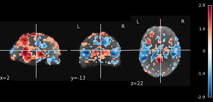
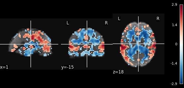
We can see that the generated components represent both signal and noise, underscoring the complex spatiotemporal patterns in real fMRI time series. For decomposition methods that are specifically tailored to fMRI data, please refer to Deriving spatial maps from group fMRI data using ICA and Dictionary Learning.

Estimated memory usage: 259 MB