BIDS dataset first- and second-level analysis

This example provides a step-by-step walk-through of fitting a first- and second-level GLM to perform massively univariate statistical analysis of a BIDS dataset, then visualizing the results. Full details about the BIDS standard can be consulted at https://bids.neuroimaging.io/.

More specifically, this example will be divided into three sections:

1. Downloading an fMRI BIDS dataset in MNI space, with two task conditions to contrast.

2. Extracting GLM first-level model objects automatically from the BIDS dataset.

3. Fitting a GLM second-level model directly from the fitted GLM first-level models.

Fetch example BIDS dataset

We download a simplified BIDS dataset made available for illustrative purposes. It contains only the necessary information for each subject to run a statistical analysis using Nilearn. Each of the raw data folders contain bold.json and events.tsv files, indicating fMRI metadata and the timing of the task events, respectively. The derivatives folders include preprocessed fMRI files preproc.nii and their accompanying confounds.tsv files.

For more information on this dataset, see the fetch_language_localizer_demo_dataset description.

from nilearn.datasets import fetch_language_localizer_demo_dataset

data = fetch_language_localizer_demo_dataset()

[fetch_language_localizer_demo_dataset] Dataset directory found: /home/runner/wo
rk/nilearn/nilearn/nilearn_data/fMRI-language-localizer-demo-dataset

We can verify the location of the dataset on disk.

print(data.data_dir)

/home/runner/work/nilearn/nilearn/nilearn_data/fMRI-language-localizer-demo-dataset

Automatically extract FirstLevelModel objects

Since BIDS datasets follow a known file structure, we can automatically infer the task structure for a given task_label using first_level_from_bids.

Specifically, first_level_from_bids will extract the fMRI images (models_run_imgs), events (models_events), and confounder regressors (model_confounds) for each subject in the dataset.

These extracted data are used to instantiate a FirstLevelModel, one for each subject. Here, these are the models objects.

from nilearn.glm.first_level import first_level_from_bids

task_label = "languagelocalizer"
(
    models,
    models_run_imgs,
    models_events,
    models_confounds,
) = first_level_from_bids(
    data.data_dir,
    task_label,
    img_filters=[("desc", "preproc")],
    n_jobs=2,
    space_label="",
    smoothing_fwhm=8,
)

/home/runner/work/nilearn/nilearn/examples/07_advanced/plot_bids_analysis.py:70: RuntimeWarning:

'StartTime' not found in file /home/runner/work/nilearn/nilearn/nilearn_data/fMRI-language-localizer-demo-dataset/derivatives/sub-01/func/sub-01_task-languagelocalizer_desc-preproc_bold.json.

/home/runner/work/nilearn/nilearn/examples/07_advanced/plot_bids_analysis.py:70: UserWarning:

'slice_time_ref' not provided and cannot be inferred from metadata.
It will be assumed that the slice timing reference is 0.0 percent of the repetition time.
If it is not the case it will need to be set manually in the generated list of models.

Quick sanity check on the extracted data

It is good practice to verify that the data extracted from the BIDS dataset is as expected. Note that Nilearn does not run an extensive BIDS validation internally.

First, we confirm that each model_run_imgs list corresponds to one subject, as expected.

from pathlib import Path

for _subject_idx, subject_runs in enumerate(models_run_imgs[:2]):
    for run in subject_runs:
        print(Path(run).name)

sub-01_task-languagelocalizer_desc-preproc_bold.nii.gz
sub-02_task-languagelocalizer_desc-preproc_bold.nii.gz

Next, we verify the column headers of the first confounds table; i.e., for the first subject.

for _subject_idx, subject_confounds in enumerate(models_confounds[:1]):
    for confounds in subject_confounds:
        print(confounds.columns)

Index(['RotX', 'RotY', 'RotZ', 'X', 'Y', 'Z'], dtype='object')

Finally, we verify the event structure. During this acquisition, each subject read blocks of sentences and consonant strings. These are the two conditions in the “languagelocalizer” task. We verify that there are 12 blocks for each condition for the first subject.

for _subject_idx, subject_events in enumerate(models_events[:1]):
    for events in subject_events:
        print(events["trial_type"].value_counts())

trial_type
language    12
string      12
Name: count, dtype: int64

For a single subject, we can visualize their event structure using plot_event.

from nilearn.plotting import plot_event

plot_event(events)

<Figure size 640x480 with 1 Axes>

First-level model estimation

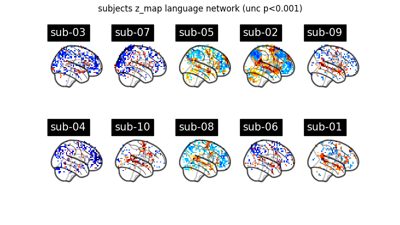
Now we simply fit each first-level GLM model each subject. We can then plot the task-specific contrast (language - string). Notice that we can define a contrast using the names of the conditions specified in the events dataframe. Sum, subtraction and scalar multiplication are allowed.

Set the threshold as the z-variate with an uncorrected p-value of 0.001.

from scipy.stats import norm

p001_unc = norm.isf(0.001)

Plot individual contrast maps.

from math import ceil

import matplotlib.pyplot as plt
import numpy as np

from nilearn import plotting

ncols = 2
nrows = ceil(len(models) / ncols)

fig, axes = plt.subplots(nrows=nrows, ncols=ncols, figsize=(10, 12))
axes = np.atleast_2d(axes)

# lists from `first_level_from_bids` are zipped together to iterate over them
model_and_args = zip(
    models, models_run_imgs, models_events, models_confounds, strict=False
)

# for each subject:
for midx, (model, imgs, events, confounds) in enumerate(model_and_args):
    # fit the GLM
    model.fit(imgs, events, confounds)
    # compute the contrast of interest
    zmap = model.compute_contrast("language - string")
    plotting.plot_glass_brain(
        zmap,
        threshold=p001_unc,
        title=f"sub-{model.subject_label}",
        axes=axes[int(midx / ncols), int(midx % ncols)],
        plot_abs=False,
        colorbar=True,
        display_mode="x",
        vmin=-12,
        vmax=12,
    )
fig.suptitle("Subjects's z_map language network (unc. p<0.001)")
plotting.show()

Second-level model estimation

Now, we just have to provide the list of fitted FirstLevelModel objects to the SecondLevelModel object for estimation. We can do this because all subjects share a similar design matrix (i.e., the same variables represented with identical column names).

from nilearn.glm.second_level import SecondLevelModel

second_level_input = models

We apply a smoothing of 8mm and parallelize the computation.

second_level_model = SecondLevelModel(smoothing_fwhm=8.0, n_jobs=2)
second_level_model = second_level_model.fit(second_level_input)

Computing contrasts at the second-level is as simple as at the first-level. Since we are not providing confounders, we are performing a one-sample test at the second-level with the images determined by the specified first-level contrast.

zmap = second_level_model.compute_contrast(
    first_level_contrast="language - string"
)

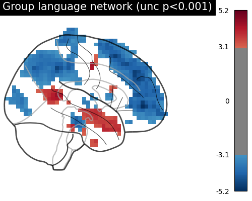
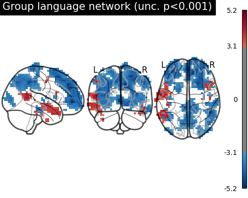
The second-level contrast reveals a left lateralized fronto-temporal language network.

plotting.plot_glass_brain(
    zmap,
    threshold=p001_unc,
    title="Group language network (unc. p<0.001)",
    plot_abs=False,
    figure=plt.figure(figsize=(5, 4)),
)
plotting.show()

We can generate and save the second-level GLM report.

report_slm = second_level_model.generate_report(
    contrasts="intercept",
    first_level_contrast="language - string",
    threshold=p001_unc,
    height_control=None,
    display_mode="x",
)

View the second-level GLM report.

Note

The generated report can be:

• displayed in a Notebook,

• opened in a browser using the .open_in_browser() method,

• or saved to a file using the .save_as_html(output_filepath) method.

report_slm

SecondLevelModel Implement the :term:`General Linear Model` for multiple subject :term:`fMRI` data.

Description

Data were analyzed using Nilearn (version= 0.14.1; RRID:SCR_001362).

At the group level, a mass univariate analysis was performed with a linear regression at each voxel of the brain.

Input images were smoothed with gaussian kernel (full-width at half maximum=8.0 mm).

The following contrasts were computed :

• intercept

Model details

	Value
Parameter
smoothing_fwhm (mm)	8.0

Design Matrix

Contrasts

Mask

The mask includes 23640 voxels (23.1 %) of the image.

Statistical Maps

intercept

Cluster Table

Height control	None
Threshold Z	3.09
Cluster size threshold (voxels)	0
Minimum distance (mm)	8.0

Cluster ID	X	Y	Z	Peak Stat	Cluster Size (mm3)
1	-57.5	-48.5	13.5	4.43	6652
1a	-71.0	-53.0	18.0	3.64
2	-62.0	-8.0	49.5	4.32	1184
2a	-53.0	-8.0	45.0	4.17
2b	-48.5	-3.5	54.0	3.16
3	-48.5	-30.5	-22.5	3.98	637
4	46.0	5.5	-27.0	3.91	3371
4a	50.5	23.5	-27.0	3.80
4b	55.0	14.5	-18.0	3.79
5	-71.0	-17.0	-4.5	3.89	9841
5a	-53.0	-8.0	-9.0	3.82
5b	-66.5	1.0	-4.5	3.82
5c	-48.5	19.0	-18.0	3.69
6	-39.5	-3.5	-40.5	3.60	455
7	50.5	-12.5	-9.0	3.51	364
8	-48.5	14.5	18.0	3.43	364
9	-75.5	-35.0	4.5	3.32	91
10	32.5	-17.0	-27.0	3.26	91
11	-44.0	-17.0	-31.5	3.13	182

About

• Date preprocessed: 2026-08-27T17:21:32

Estimated memory usage: 402 MB