Tuning a parameter with cross-validation

This example presents a nested cross-validation (CV) approach to perform hyperparameter tuning and model performance evaluation with Decoder objects.

The Decoder is a composite estimator that:

1. Applies a masker to the input images

2. Performs ANOVA univariate feature selection

3. Fits a classifier to the preprocessed data.

More information about the inner workings of the Decoder class can be found at this page.

The Decoder class implements a model selection scheme that averages the best models within a cross-validation loop (a technique sometimes known as CV bagging). However, there is no built-in way to tune hyperparameters related to feature selection: this has to be done manually using the nested cross-validation method, where the inner CV loop is used to tune hyperparameters and the outer CV loop is used to evaluate model performance. See https://scikit-learn.org/stable/modules/cross_validation.html for an excellent explanation of how cross-validation works.

import warnings

warnings.filterwarnings(
    "ignore", message="The provided image has no sform in its header."
)

# set overall verbosity for this example
verbose = 0

Load the Haxby dataset

We start by loading fMRI data and target labels from the Haxby dataset.

import pandas as pd

from nilearn import datasets
from nilearn.image import index_img

# load data from a single subject
haxby_dataset = datasets.fetch_haxby(verbose=verbose)
fmri_img = haxby_dataset.func[0]
mask_img = haxby_dataset.mask

print(f"Mask nifti image (3D) is located at: {haxby_dataset.mask}")
print(f"Functional nifti image (4D) are located at: {haxby_dataset.func[0]}")

# Load the behavioral data
labels = pd.read_csv(haxby_dataset.session_target[0], sep=" ")
y = labels["labels"]

# Keep only data corresponding to shoes or bottles
condition_mask = y.isin(["shoe", "bottle"])
fmri_niimgs = index_img(fmri_img, condition_mask)
y = y[condition_mask]
runs = labels["chunks"][condition_mask]  # 12 runs total

Mask nifti image (3D) is located at: /home/runner/nilearn_data/haxby2001/mask.nii.gz
Functional nifti image (4D) are located at: /home/runner/nilearn_data/haxby2001/subj2/bold.nii.gz

Tuning the screening_percentile parameter

The rest of this example will consist of a step-by-step walkthrough of how to tune a feature selection hyperparameter, screening_percentile. For the full nested cross-validation (best practice) approach, see the end of this page.

Helper function

Let’s define a helper function that creates and fits a single instance of a Decoder with a given value of the screening_percentile parameter. This function will allow us to avoid duplication of the code since we only want to vary the screening_percentile hyperparameter.

import warnings

from nilearn.decoding import Decoder


def fit_decoder(X, y, screening_percentile, verbose=0):
    decoder = Decoder(
        estimator="svc",
        cv=3,
        mask=mask_img,  # previously loaded, same for all decoders
        smoothing_fwhm=4,
        screening_percentile=screening_percentile,
        verbose=verbose,
    )
    decoder.fit(X, y)
    return decoder

Trying different values of the screening_percentile hyperparameter

Here we fit the decoder on a subset of the data (the first 10 runs) using different values for the screening_percentile parameter. We can see which screening percentile gives the best validation score.

screening_percentiles = [2, 4, 8, 16, 32, 64]

idx_train = runs < 10  # first 10 runs
idx_val = ~idx_train  # remaining 2 runs

X_train = index_img(fmri_niimgs, idx_train)
y_train = y[idx_train]
X_val = index_img(fmri_niimgs, idx_val)
y_val = y[idx_val]

validation_scores = {}  # {screening_percentile: validation_score}
for screening_percentile in screening_percentiles:
    decoder = fit_decoder(
        X_train,
        y_train,
        screening_percentile=screening_percentile,
        verbose=verbose,
    )
    validation_scores[screening_percentile] = decoder.score(X_val, y_val)

print("\nValidation scores:")
for screening_percentile, val_score in validation_scores.items():
    print(f"- {screening_percentile=}: {val_score:.4f}")

Validation scores:
- screening_percentile=2: 0.6358
- screening_percentile=4: 0.6173
- screening_percentile=8: 0.6049
- screening_percentile=16: 0.5864
- screening_percentile=32: 0.5556
- screening_percentile=64: 0.5741

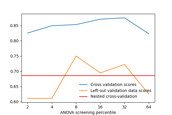
The above block of code can help determine which screening percentile is optimal when the decoder is fitted and validated on specific data. However, there are some important caveats to note:

1. The above code use a single train-test split. Different splits will give different validation scores, and it is possible that the best screening percentile is different for different splits.

2. The validation score should not be used as an estimate of the generalization performance of the model, since validation data was used to select the best screening percentile (in other words, it is not truly held-out data).

These points are addressed by using nested cross-validation.

Full nested cross-validation

Nested cross-validation works as follows:

1. The inner CV loop is used for hyperparameter tuning. Multiple validation scores are obtained for each value of the hyperparameter, and the best value is selected based on the average validation score across folds. Note: this is similar in concept to sklearn’s GridSearchCV, which cannot be used here because of input data incompatibility between the Decoder class and other sklearn estimators.

2. The outer CV loop is used for model evaluation. For each fold, the model is refit using the best hyperparameter value from the inner CV loop, and a test score is obtained on the left-out test set. We then report the average test score across folds as an estimate of the generalization performance of the model.

   In addition, we plot the average validation scores across inner CV folds for each value of the hyperparameter. This can help us visualize the hyperparameter tuning process and the stability of the best hyperparameter value across different outer CV folds.

import matplotlib.pyplot as plt
import numpy as np
from sklearn.model_selection import GroupKFold

plt.figure(figsize=(6, 4))
plt.xticks(np.arange(len(screening_percentiles)), screening_percentiles)
plt.xlabel("ANOVA screening percentile")
plt.ylabel("Average validation score across inner CV folds")

outer_cv = GroupKFold(n_splits=3)
test_scores = []

# outer CV loop for model evaluation
# the test set here are left out from the entire model fitting and
# selection process
for idx_train_val, idx_test in outer_cv.split(
    np.arange(len(runs)), groups=runs
):
    # inner CV loop for hyperparameter tuning
    # the train set is used to fit the model and the validation set is used to
    # select the best screening percentile for this CV split
    mean_val_scores = {}
    for screening_percentile in screening_percentiles:
        inner_cv = GroupKFold(n_splits=3)
        val_scores = []
        for idx_train, idx_val in inner_cv.split(
            idx_train_val, groups=runs.iloc[idx_train_val]
        ):
            # inner_cv.split() returns indices relative to idx_train_val, so we
            # need to index into idx_train_val to get the actual indices for
            # the train and validation sets
            idx_train = idx_train_val[idx_train]
            idx_val = idx_train_val[idx_val]

            X_train = index_img(fmri_niimgs, idx_train)
            y_train = y.iloc[idx_train]
            X_val = index_img(fmri_niimgs, idx_val)
            y_val = y.iloc[idx_val]

            decoder = fit_decoder(
                X_train,
                y_train,
                screening_percentile=screening_percentile,
                verbose=verbose,
            )
            val_scores.append(decoder.score(X_val, y_val))

        mean_val_scores[screening_percentile] = np.mean(val_scores)

    best_screening_percentile = max(mean_val_scores, key=mean_val_scores.get)

    # plot average validation score for each screening percentile value
    # use a different marker shape for the best screening percentile
    i_fold = len(test_scores)
    color = f"C{i_fold}"
    plt.scatter(
        np.arange(len(screening_percentiles)),
        mean_val_scores.values(),
        c=[
            color
            if screening_percentile != best_screening_percentile
            else "white"
            for screening_percentile in screening_percentiles
        ],
        label=f"Outer CV fold {i_fold + 1}",
    )
    plt.scatter(
        screening_percentiles.index(best_screening_percentile),
        mean_val_scores[best_screening_percentile],
        c=color,
        s=100,
        marker="*",
    )

    # pick the best screening percentile from the inner CV loop
    print("Average validation scores by screening percentile:")
    for screening_percentile, score in mean_val_scores.items():
        str_best = ""
        if screening_percentile == best_screening_percentile:
            str_best = " (best)"
        print(f"{screening_percentile=}:\t{score:.4f}{str_best}")

    # refit the model and evaluate on the test set
    X_train_val = index_img(fmri_niimgs, idx_train_val)
    y_train_val = y.iloc[idx_train_val]
    X_test = index_img(fmri_niimgs, idx_test)
    y_test = y.iloc[idx_test]

    decoder = fit_decoder(
        X_train_val,
        y_train_val,
        screening_percentile=best_screening_percentile,
        verbose=verbose,
    )
    test_scores.append(decoder.score(X_test, y_test))

plt.legend()

# final model performance estimation
print(
    "Mean ± std test score:\t"
    f"{np.mean(test_scores):.4f} ± {np.std(test_scores):.4f}"
)

Average validation scores by screening percentile:
screening_percentile=2: 0.5941
screening_percentile=4: 0.6035 (best)
screening_percentile=8: 0.6032
screening_percentile=16:        0.5740
screening_percentile=32:        0.5751
screening_percentile=64:        0.5854
Average validation scores by screening percentile:
screening_percentile=2: 0.5526
screening_percentile=4: 0.5780 (best)
screening_percentile=8: 0.5584
screening_percentile=16:        0.4809
screening_percentile=32:        0.4751
screening_percentile=64:        0.4720
Average validation scores by screening percentile:
screening_percentile=2: 0.5568
screening_percentile=4: 0.5585
screening_percentile=8: 0.5740
screening_percentile=16:        0.5730
screening_percentile=32:        0.5720
screening_percentile=64:        0.5757 (best)
Mean ± std test score:  0.6880 ± 0.0481

Estimated memory usage: 1002 MB