Comparing connectomes on different reference atlases

This example shows how to turn a parcellation into connectome for visualization. This requires choosing centers for each parcel or network, via find_parcellation_cut_coords for parcellation based on deterministic atlases (labels) and find_probabilistic_atlas_cut_coords for parcellation based on probabilistic atlases (maps).

In the intermediary steps, we make use of MultiNiftiLabelsMasker and MultiNiftiMapsMasker to extract time series from nifti objects representing multiple subjects using different parcellation atlases.

The time series of all subjects of the brain development dataset are concatenated and given directly to ConnectivityMeasure for computing parcel-wise correlation matrices for each atlas across all subjects.

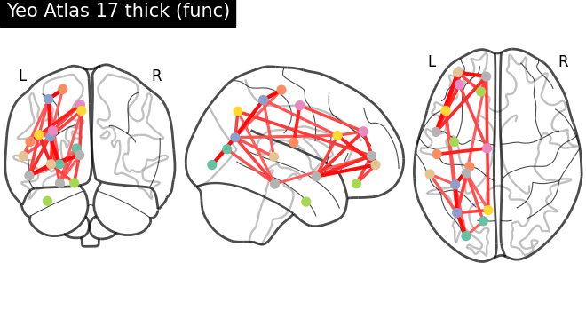
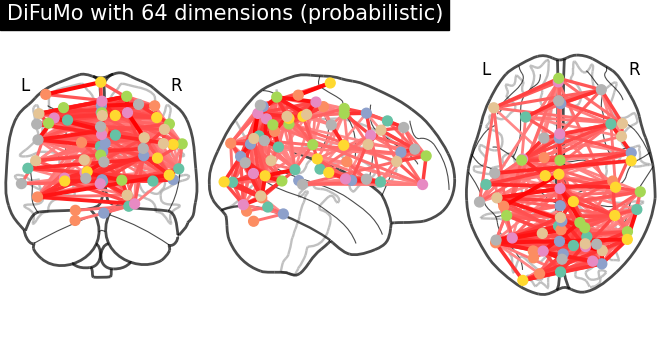
Mean correlation matrix is displayed on glass brain on extracted coordinates.

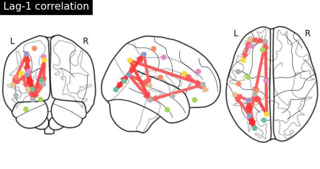
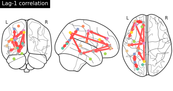
The example also covers a special case of plotting directed connectome, such as results from Granger causality. To demonstrate the utility, we created an asymmetric connectome, which would be similar to results from Granger causality.

# control overall verbosity of the script
verbose = 0

Load functional data

from nilearn.datasets import fetch_development_fmri

data = fetch_development_fmri(n_subjects=10)

print(
    "Functional nifti images (4D, e.g., one subject) "
    f"are located at : {data.func[0]!r}"
)
print(
    "Counfound csv files (of same subject) are located "
    f"at : {data.confounds[0]!r}"
)

[fetch_development_fmri] Dataset directory found: /home/runner/work/nilearn/nilearn/nilearn_data/development_fmri
Functional nifti images (4D, e.g., one subject) are located at : '/home/runner/work/nilearn/nilearn/nilearn_data/development_fmri/sub-pixar123_task-pixar_space-MNI152NLin2009cAsym_desc-preproc_bold.nii.gz'
Counfound csv files (of same subject) are located at : '/home/runner/work/nilearn/nilearn/nilearn_data/development_fmri/sub-pixar123_task-pixar_desc-reducedConfounds_regressors.tsv'

Extract coordinates from a deterministic parcellation - Yeo atlas

For this first section we are using the Yeo atlas.

from nilearn.connectome import ConnectivityMeasure
from nilearn.datasets import fetch_atlas_yeo_2011
from nilearn.maskers import MultiNiftiLabelsMasker

yeo = fetch_atlas_yeo_2011(n_networks=17)
print(
    "Yeo atlas nifti image (3D) with 17 parcels and liberal mask "
    f" is located at: {yeo['maps']}"
)

# ConnectivityMeasure from Nilearn uses simple 'correlation' to compute
# connectivity matrices for all subjects in a list.
connectome_measure = ConnectivityMeasure(kind="correlation", verbose=verbose)

# create masker using MultiNiftiLabelsMasker to extract functional data within
# atlas parcels from multiple subjects using parallelization to speed up the
# computation
masker = MultiNiftiLabelsMasker(
    labels_img=yeo["maps"],  # Both hemispheres,
    standardize="zscore_sample",
    standardize_confounds=True,
    memory="nilearn_cache",
    n_jobs=2,
    verbose=verbose,
)

# extract time series from all subjects
time_series = masker.fit_transform(data.func, confounds=data.confounds)

# calculate correlation matrices across subjects and display
correlation_matrices = connectome_measure.fit_transform(time_series)

# Mean correlation matrix across 10 subjects can be grabbed like this,
# using connectome measure object
mean_correlation_matrix = connectome_measure.mean_

# useful for plotting connectivity interactions on glass brain
from nilearn.plotting import (
    find_parcellation_cut_coords,
    plot_connectome,
    show,
)

# grab center coordinates for atlas labels
coordinates = find_parcellation_cut_coords(labels_img=yeo["maps"])

# plot connectome with 80% edge strength in the connectivity
left_connectome = plot_connectome(
    mean_correlation_matrix, coordinates, edge_threshold="80%"
)

show()

[fetch_atlas_yeo_2011] Dataset directory found: /home/runner/work/nilearn/nilearn/nilearn_data/yeo_2011
Yeo atlas nifti image (3D) with 17 parcels and liberal mask  is located at: /home/runner/work/nilearn/nilearn/nilearn_data/yeo_2011/Yeo_JNeurophysiol11_MNI152/Yeo2011_17Networks_MNI152_FreeSurferConformed1mm_LiberalMask.nii.gz
/home/runner/work/nilearn/nilearn/.tox/doc/lib/python3.11/site-packages/joblib/externals/loky/process_executor.py:782: UserWarning:

A worker stopped while some jobs were given to the executor. This can be caused by a too short worker timeout or by a memory leak.

Note

The approach above will extract time series and compute a single connectivity matrix for both hemispheres. However, the connectome is plotted only for the left hemisphere.

If your aim is to compute and plot hemisphere-wise connectivity, you can follow the example below.

First, create a separate atlas image for each hemisphere:

import nibabel as nb
import numpy as np

from nilearn.image import coord_transform, get_data, new_img_like

# load the atlas image first
label_image = nb.load(yeo["maps"])

# extract the affine matrix of the image
labels_affine = label_image.affine

# generate image coordinates using affine
x, y, z = coord_transform(0, 0, 0, np.linalg.inv(labels_affine))

# generate a separate image for the left hemisphere
# left/right split is done along x-axis
left_hemi = get_data(label_image).copy()
left_hemi[: int(x)] = 0
label_image_left = new_img_like(label_image, left_hemi, labels_affine)

# same for the right hemisphere
right_hemi = get_data(label_image).copy()
right_hemi[int(x) :] = 0
label_image_right = new_img_like(label_image, right_hemi, labels_affine)

Then, create a masker object, compute a connectivity matrix and plot the results for each hemisphere:

for hemi, img in zip(
    ["right", "left"], [label_image_right, label_image_left], strict=False
):
    masker = MultiNiftiLabelsMasker(
        labels_img=img,
        standardize="zscore_sample",
        standardize_confounds=True,
        verbose=verbose,
    )

    time_series = masker.fit_transform(data.func, confounds=data.confounds)

    correlation_matrices = connectome_measure.fit_transform(time_series)
    mean_correlation_matrix = connectome_measure.mean_

    coordinates = find_parcellation_cut_coords(
        labels_img=img, label_hemisphere=hemi
    )

    plot_connectome(
        mean_correlation_matrix,
        coordinates,
        edge_threshold="80%",
        title=f"Yeo Atlas 17 thick (func) - {hemi}",
    )

show()

• 
• 

Plot a directed connectome - asymmetric connectivity measure

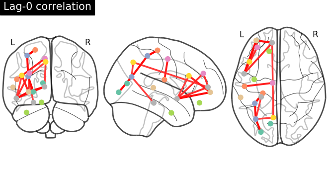
In this section, we use the lag-1 correlation as the connectivity measure, which leads to an asymmetric connectivity matrix. The plot_connectome function accepts both symmetric and asymmetric matrices, but plots the latter as a directed graph.

# Define a custom function to compute lag correlation on the time series
def lag_correlation(time_series, lag):
    n_subjects = len(time_series)
    _, n_features = time_series[0].shape
    lag_cor = np.zeros((n_subjects, n_features, n_features))
    for subject, serie in enumerate(time_series):
        for i in range(n_features):
            for j in range(n_features):
                if lag == 0:
                    lag_cor[subject, i, j] = np.corrcoef(
                        serie[:, i], serie[:, j]
                    )[0, 1]
                else:
                    lag_cor[subject, i, j] = np.corrcoef(
                        serie[lag:, i], serie[:-lag, j]
                    )[0, 1]
    return np.mean(lag_cor, axis=0)


# Compute lag-0 and lag-1 correlations and plot associated connectomes
for lag in [0, 1]:
    lag_correlation_matrix = lag_correlation(time_series, lag)
    plot_connectome(
        lag_correlation_matrix,
        coordinates,
        edge_threshold="90%",
        title=f"Lag-{lag} correlation",
    )

• 
• 

/home/runner/work/nilearn/nilearn/examples/03_connectivity/plot_atlas_comparison.py:213: UserWarning:

'adjacency_matrix' is not symmetric.
A directed graph will be plotted.

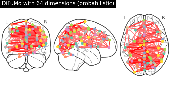
Extract coordinates from a probabilistic parcellation - Difumo atlas

For this second section we are using the Difumo atlas.

from nilearn.datasets import fetch_atlas_difumo
from nilearn.plotting import find_probabilistic_atlas_cut_coords

dim = 64
difumo = fetch_atlas_difumo(dimension=dim, resolution_mm=2)

[fetch_atlas_difumo] Dataset directory found: /home/runner/work/nilearn/nilearn/nilearn_data/difumo_atlases

Iterate over fetched atlases to extract coordinates - probabilistic

from nilearn.maskers import MultiNiftiMapsMasker

# Create masker using MultiNiftiMapsMasker to extract functional data within
# atlas parcels from multiple subjects using parallelization to speed up the
# computation.
masker = MultiNiftiMapsMasker(
    maps_img=difumo.maps,
    standardize="zscore_sample",
    standardize_confounds=True,
    memory="nilearn_cache",
    memory_level=1,
    n_jobs=2,
    verbose=verbose,
)

# extract time series from all subjects
time_series = masker.fit_transform(data.func, confounds=data.confounds)

# calculate correlation matrices across subjects and display
correlation_matrices = connectome_measure.fit_transform(time_series)

# Mean correlation matrix across 10 subjects can be grabbed like this,
# using connectome measure object
mean_correlation_matrix = connectome_measure.mean_

# grab center coordinates for probabilistic atlas
coordinates = find_probabilistic_atlas_cut_coords(maps_img=difumo.maps)

# plot connectome with 85% edge strength in the connectivity
plot_connectome(
    mean_correlation_matrix,
    coordinates,
    edge_threshold="85%",
    title=f"DiFuMo with {dim} dimensions (probabilistic)",
)
show()

Estimated memory usage: 3088 MB