Analysis of an fMRI dataset with a Finite Impule Response (FIR) model

FIR models are used to estimate the hemodyamic response non-parametrically. The example below shows that they’re good to do statistical inference even on fast event-related fMRI datasets.

Here, we demonstrate the use of a FIR model with 3 lags, computing 4 contrasts from a single subject dataset from the “Neurospin Localizer”.

See also

For more information about the dataset see its description.

At first, we grab the localizer data.

import pandas as pd

from nilearn.datasets import func
from nilearn.plotting import plot_stat_map

data = func.fetch_localizer_first_level()
fmri_img = data.epi_img
t_r = data.t_r
events_file = data["events"]
events = pd.read_table(events_file)

[fetch_localizer_first_level] Dataset directory found:
/home/runner/nilearn_data/localizer_first_level

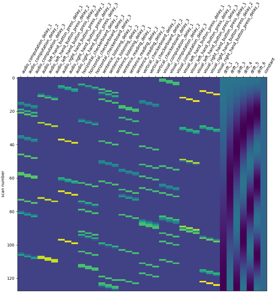
Next solution is to try Finite Impulse Response (FIR) models: we just say that the hrf is an arbitrary function that lags behind the stimulus onset. In the present case, given that the numbers of conditions is high, we should use a simple FIR model.

Concretely, we set hrf_model to ‘fir’ and fir_delays to [1, 2, 3] (scans) corresponding to a 3-step functions on the [1 * t_r, 4 * t_r] seconds interval.

from nilearn.glm.first_level import FirstLevelModel
from nilearn.plotting import plot_contrast_matrix, plot_design_matrix

first_level_model = FirstLevelModel(
    t_r, hrf_model="fir", fir_delays=[1, 2, 3], verbose=1
)
first_level_model = first_level_model.fit(fmri_img, events=events)
design_matrix = first_level_model.design_matrices_[0]
plot_design_matrix(design_matrix)

\[FirstLevelModel.fit] Computing run 1 out of 1 runs (go take a coffee, a big
one).
\[FirstLevelModel.fit] Performing mask computation.
\[FirstLevelModel.fit] Masking took 0 seconds.
\[FirstLevelModel.fit] Performing GLM computation.
\[FirstLevelModel.fit] GLM took 1 seconds.
\[FirstLevelModel.fit] Computation of 1 runs done in 00 HR 00 MIN 02 SEC.

<Axes: label='conditions', ylabel='scan number'>

We have to adapt contrast specification. We characterize the BOLD response by the sum across the three time lags. It’s a bit hairy, sorry, but this is the price to pay for flexibility…

import numpy as np

contrast_matrix = np.eye(design_matrix.shape[1])
contrasts = {
    column: contrast_matrix[i]
    for i, column in enumerate(design_matrix.columns)
}
conditions = events.trial_type.unique()
for condition in conditions:
    contrasts[condition] = np.sum(
        [
            contrasts[name]
            for name in design_matrix.columns
            if name[: len(condition)] == condition
        ],
        0,
    )

contrasts["audio"] = np.sum(
    [
        contrasts[name]
        for name in [
            "audio_right_hand_button_press",
            "audio_left_hand_button_press",
            "audio_computation",
            "sentence_listening",
        ]
    ],
    0,
)
contrasts["video"] = np.sum(
    [
        contrasts[name]
        for name in [
            "visual_right_hand_button_press",
            "visual_left_hand_button_press",
            "visual_computation",
            "sentence_reading",
        ]
    ],
    0,
)

contrasts["computation"] = (
    contrasts["audio_computation"] + contrasts["visual_computation"]
)
contrasts["sentences"] = (
    contrasts["sentence_listening"] + contrasts["sentence_reading"]
)

contrasts = {
    "left-right": (
        contrasts["visual_left_hand_button_press"]
        + contrasts["audio_left_hand_button_press"]
        - contrasts["visual_right_hand_button_press"]
        - contrasts["audio_right_hand_button_press"]
    ),
    "H-V": (
        contrasts["horizontal_checkerboard"]
        - contrasts["vertical_checkerboard"]
    ),
    "audio-video": contrasts["audio"] - contrasts["video"],
    "sentences-computation": (
        contrasts["sentences"] - contrasts["computation"]
    ),
}

Take a look at the contrasts.

plot_contrast_matrix(contrasts["left-right"], design_matrix)

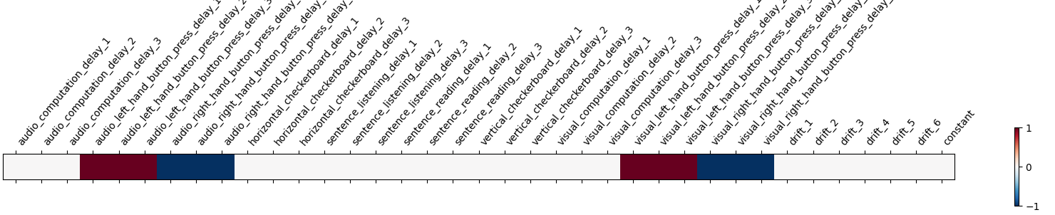
<Axes: label='conditions'>

Take a breath.

We can now proceed by estimating the contrasts and displaying them.

import matplotlib.pyplot as plt

fig = plt.figure(figsize=(11, 3))
for index, (contrast_id, contrast_val) in enumerate(contrasts.items()):
    ax = plt.subplot(1, len(contrasts), 1 + index)
    z_map = first_level_model.compute_contrast(
        contrast_val, output_type="z_score"
    )
    plot_stat_map(
        z_map,
        display_mode="z",
        threshold=3.0,
        title=contrast_id,
        axes=ax,
        cut_coords=1,
    )
plt.show()

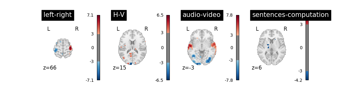
The result is acceptable. Note that we’re asking a lot of questions to a small dataset, yet with a relatively large number of experimental conditions.

Estimated memory usage: 355 MB