Example of pattern recognition on simulated data

This example simulates data according to a very simple sketch of brain imaging data and applies machine learning techniques to predict output values.

We use a very simple generating function to simulate data, as in Michel et al.[1], a linear model with a random design matrix X:

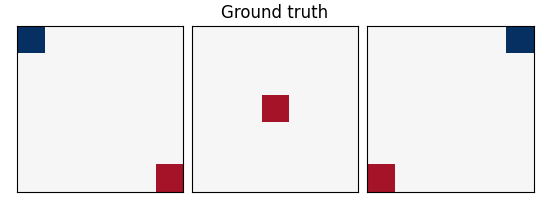
• w: the weights of the linear model correspond to the predictive brain regions. Here, in the simulations, they form a 3D image with 5, four of which in opposite corners and one in the middle, as plotted below.

• X: the design matrix corresponds to the observed fMRI data. Here we simulate random normal variables and smooth them as in Gaussian fields.

• e is random normal noise.

from nilearn._utils.helpers import check_matplotlib

check_matplotlib()

from time import time

import matplotlib.pyplot as plt
import numpy as np
from nibabel import Nifti1Image
from scipy import linalg
from scipy.ndimage import gaussian_filter
from sklearn import linear_model, svm
from sklearn.feature_selection import f_regression
from sklearn.model_selection import KFold
from sklearn.pipeline import make_pipeline
from sklearn.preprocessing import StandardScaler
from sklearn.utils import check_random_state

import nilearn.masking
from nilearn import decoding
from nilearn.plotting import show

A function to generate data

def create_simulation_data(snr=0, n_samples=2 * 100, size=12, random_state=1):
    generator = check_random_state(random_state)
    roi_size = 2  # size / 3
    smooth_X = 1
    # Coefs
    w = np.zeros((size, size, size))
    w[0:roi_size, 0:roi_size, 0:roi_size] = -0.6
    w[-roi_size:, -roi_size:, 0:roi_size] = 0.5
    w[0:roi_size, -roi_size:, -roi_size:] = -0.6
    w[-roi_size:, 0:roi_size:, -roi_size:] = 0.5
    w[
        (size - roi_size) // 2 : (size + roi_size) // 2,
        (size - roi_size) // 2 : (size + roi_size) // 2,
        (size - roi_size) // 2 : (size + roi_size) // 2,
    ] = 0.5
    w = w.ravel()
    # Generate smooth background noise
    XX = generator.randn(n_samples, size, size, size)
    noise = []
    for i in range(n_samples):
        Xi = gaussian_filter(XX[i, :, :, :], smooth_X)
        Xi = Xi.ravel()
        noise.append(Xi)
    noise = np.array(noise)
    # Generate the signal y
    y = generator.randn(n_samples)
    X = np.dot(y[:, np.newaxis], w[np.newaxis])
    norm_noise = linalg.norm(X, 2) / np.exp(snr / 20.0)
    noise_coef = norm_noise / linalg.norm(noise, 2)
    noise *= noise_coef
    snr = 20 * np.log(linalg.norm(X, 2) / linalg.norm(noise, 2))
    print(f"SNR: {snr:.1f} dB")
    # Mixing of signal + noise and splitting into train/test
    X += noise
    X -= X.mean(axis=-1)[:, np.newaxis]
    X /= X.std(axis=-1)[:, np.newaxis]
    X_test = X[n_samples // 2 :, :]
    X_train = X[: n_samples // 2, :]
    y_test = y[n_samples // 2 :]
    y = y[: n_samples // 2]

    return X_train, X_test, y, y_test, snr, w, size

A simple function to plot slices

def plot_slices(data, title=None):
    plt.figure(figsize=(5.5, 2.2))
    vmax = np.abs(data).max()
    for i in (0, 6, 11):
        plt.subplot(1, 3, i // 5 + 1)
        plt.imshow(
            data[:, :, i],
            vmin=-vmax,
            vmax=vmax,
            interpolation="nearest",
            cmap="RdBu_r",
        )
        plt.xticks(())
        plt.yticks(())
    plt.subplots_adjust(
        hspace=0.05, wspace=0.05, left=0.03, right=0.97, top=0.9
    )
    if title is not None:
        plt.suptitle(title)

Create data

X_train, X_test, y_train, y_test, snr, coefs, size = create_simulation_data(
    snr=-10, n_samples=100, size=12
)

# Create masks for SearchLight. process_mask is the voxels where SearchLight
# computation is performed. It is a subset of the brain mask, just to reduce
# computation time.
mask = np.ones((size, size, size), dtype=bool)
mask_img = Nifti1Image(mask.astype("uint8"), np.eye(4))
process_mask = np.zeros((size, size, size), dtype=bool)
process_mask[:, :, 0] = True
process_mask[:, :, 6] = True
process_mask[:, :, 11] = True
process_mask_img = Nifti1Image(process_mask.astype("uint8"), np.eye(4))

coefs = np.reshape(coefs, [size, size, size])
plot_slices(coefs, title="Ground truth")

SNR: -10.0 dB

Run different estimators

We can now run different estimators and look at their prediction score, as well as the feature maps that they recover. Namely, we will use

• A support vector regression

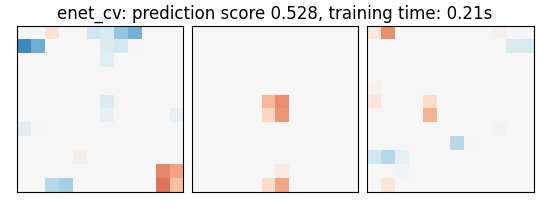
• An elastic-net

• A Bayesian ridge estimator, i.e. a ridge estimator that sets its parameter according to a metaprior

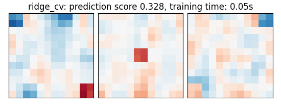
• A ridge estimator that set its parameter by cross-validation

Note that the RidgeCV and the ElasticNetCV have names ending in CV that stands for cross-validation: in the list of possible alpha values that they are given, they choose the best by cross-validation.

bayesian_ridge = make_pipeline(StandardScaler(), linear_model.BayesianRidge())

estimators = [
    ("bayesian_ridge", bayesian_ridge),
    (
        "enet_cv",
        linear_model.ElasticNetCV(alphas=[5, 1, 0.5, 0.1], l1_ratio=0.05),
    ),
    ("ridge_cv", linear_model.RidgeCV(alphas=[100, 10, 1, 0.1], cv=5)),
    ("svr", svm.SVR(kernel="linear", C=0.001)),
    (
        "searchlight",
        decoding.SearchLight(
            mask_img,
            process_mask_img=process_mask_img,
            radius=2.7,
            scoring="r2",
            estimator=svm.SVR(kernel="linear"),
            cv=KFold(n_splits=4),
            verbose=1,
            n_jobs=2,
        ),
    ),
]

Run the estimators

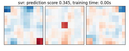
As the estimators expose a fairly consistent API, we can all fit them in a for loop: they all have a fit method for fitting the data, a score method to retrieve the prediction score, and because they are all linear models, a coef_ attribute that stores the coefficients w estimated

for name, estimator in estimators:
    t1 = time()
    if name != "searchlight":
        estimator.fit(X_train, y_train)
    else:
        X = nilearn.masking.unmask(X_train, mask_img)
        estimator.fit(X, y_train)
        del X
    elapsed_time = time() - t1

    if name != "searchlight":
        if name == "bayesian_ridge":
            coefs = estimator.named_steps["bayesianridge"].coef_
        else:
            coefs = estimator.coef_
        coefs = np.reshape(coefs, [size, size, size])
        score = estimator.score(X_test, y_test)
        title = (
            f"{name}: prediction score {score:.3f}, "
            f"training time: {elapsed_time:.2f}s"
        )

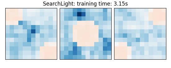
    else:  # Searchlight
        coefs = estimator.scores_
        title = (
            f"{estimator.__class__.__name__}: "
            f"training time: {elapsed_time:.2f}s"
        )

    # We use the plot_slices function provided in the example to
    # plot the results
    plot_slices(coefs, title=title)

    print(title)

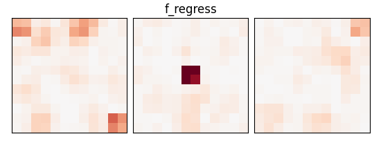
_, p_values = f_regression(X_train, y_train)
p_values = np.reshape(p_values, (size, size, size))
p_values = -np.log10(p_values)
p_values[np.isnan(p_values)] = 0
p_values[p_values > 10] = 10
plot_slices(p_values, title="f_regress")

show()

• 
• 
• 
• 
• 
• 

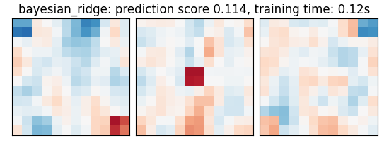
bayesian_ridge: prediction score 0.114, training time: 0.17s
enet_cv: prediction score 0.528, training time: 0.23s
ridge_cv: prediction score 0.328, training time: 0.05s
svr: prediction score 0.345, training time: 0.00s
[Parallel(n_jobs=2)]: Using backend LokyBackend with 2 concurrent workers.
[Parallel(n_jobs=2)]: Done   2 out of   2 | elapsed:    3.1s remaining:    0.0s
[Parallel(n_jobs=2)]: Done   2 out of   2 | elapsed:    3.1s finished
SearchLight: training time: 3.80s

An exercise to go further

As an exercise, you can use recursive feature elimination (RFE) with the SVM

Read the object’s documentation to find out how to use RFE.

Performance tip: increase the step parameter, or it will be very slow.

# from sklearn.feature_selection import RFE

References

[1]

Vincent Michel, Alexandre Gramfort, Gaël Varoquaux, Evelyn Eger, and Bertrand Thirion. Total variation regularization for fMRI-based prediction of behaviour. IEEE Transactions on Medical Imaging, 30(7):1328 – 1340, February 2011. URL: https://inria.hal.science/inria-00563468, doi:10.1109/TMI.2011.2113378.

Estimated memory usage: 108 MB