Note
Go to the end to download the full example code. or to run this example in your browser via Binder
Simple example of two-runs fMRI model fitting
Here, we will go through a full step-by-step example of fitting a GLM to experimental data and visualizing the results. This is done on two runs of one subject of the FIAC dataset.
Here are the steps we will go through:
Set up the GLM
Compare run-specific and fixed effects contrasts
Compute a range of contrasts across both runs
Generate a report
Technically, this example shows how to handle two runs that contain the same experimental conditions. The model directly returns a fixed effect of the statistics across the two runs.
See also
See the dataset description for more information on the data used in this example.
Create an output results in the current working directory.
from pathlib import Path

output_dir = Path.cwd() / "results" / "plot_two_runs_model"
output_dir.mkdir(exist_ok=True, parents=True)
print(f"Output will be saved to: {output_dir}")
Output will be saved to: /home/runner/work/nilearn/nilearn/examples/04_glm_first_level/results/plot_two_runs_model
Set up the GLM
Inspecting ‘data’, we note that there are two runs. We will retain those two runs in a list of 4D img objects.
from nilearn.datasets.func import fetch_fiac_first_level

data = fetch_fiac_first_level()
fmri_imgs = [data["func1"], data["func2"]]
[fetch_fiac_first_level] Dataset directory found:
/home/runner/work/nilearn/nilearn/nilearn_data/fiac_nilearn.glm
Create a mean image for plotting purpose.
The design matrices were pre-computed, we simply put them in a list of DataFrames.
import numpy as np

design_matrices = [data["design_matrix1"], data["design_matrix2"]]
Initialize and run the GLM
First, we need to specify the model before fitting it to the data. Note that a brain mask was provided in the dataset, so that is what we will use.
from nilearn.glm.first_level import FirstLevelModel

fmri_glm = FirstLevelModel(
    mask_img=data["mask"], smoothing_fwhm=5, minimize_memory=True, verbose=1
)
Compare run-specific and fixed effects contrasts
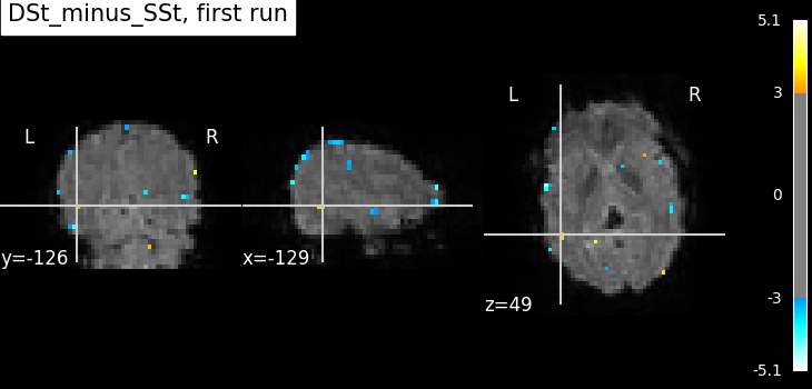
We can then compare run-specific and fixed effects. Here, we compare the activation produced from each run separately and then the fixed effects version.
contrast_id = "DSt_minus_SSt"
Compute the statistics for the first run.
Here, we define the contrast of interest for the first run. This may differ across runs depending on if the design matrices vary.
from nilearn.plotting import plot_stat_map, show

contrast_val = [[-1, -1, 1, 1]]

fmri_glm_run_1 = fmri_glm.fit(fmri_imgs[0], design_matrices=design_matrices[0])
summary_statistics_run_1 = fmri_glm_run_1.compute_contrast(
    contrast_val,
    output_type="all",
)

# Let's use the same plotting range and slices for all plots.
threshold = 3
vmax = 6.0
cut_coords = [-129, -126, 49]

plot_stat_map(
    summary_statistics_run_1["z_score"],
    bg_img=mean_img_,
    threshold=threshold,
    cut_coords=cut_coords,
    title=f"{contrast_id}, first run",
    vmax=vmax,
)

show()
/home/runner/work/nilearn/nilearn/examples/04_glm_first_level/plot_two_runs_model.py:90: RuntimeWarning:

[MultiNiftiMasker.fit] Generation of a mask has been requested (imgs != None) while a mask was given at masker creation. Given mask will be used.

\[FirstLevelModel.fit] Computing run 1 out of 1 runs (go take a coffee, a big
one).
\[FirstLevelModel.fit] Performing mask computation.
\[FirstLevelModel.fit] Masking took 1 seconds.
\[FirstLevelModel.fit] Performing GLM computation.
\[FirstLevelModel.fit] GLM took 0 seconds.
\[FirstLevelModel.fit] Computation of 1 runs done in 00 HR 00 MIN 02 SEC.
/home/runner/work/nilearn/nilearn/examples/04_glm_first_level/plot_two_runs_model.py:91: UserWarning:

t contrasts should be of length P=13, but it has length 4. The rest of the contrast was padded with zeros.
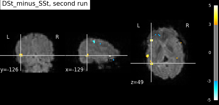
Compute the statistics for the second run.
fmri_glm_run_2 = fmri_glm.fit(fmri_imgs[1], design_matrices=design_matrices[1])

contrast_val = np.array([[-1, -1, 1, 1]])

summary_statistics_run_2 = fmri_glm_run_2.compute_contrast(
    contrast_val,
    output_type="all",
)
plot_stat_map(
    summary_statistics_run_2["z_score"],
    bg_img=mean_img_,
    threshold=threshold,
    cut_coords=cut_coords,
    title=f"{contrast_id}, second run",
    vmax=vmax,
)

show()
/home/runner/work/nilearn/nilearn/examples/04_glm_first_level/plot_two_runs_model.py:114: RuntimeWarning:

[MultiNiftiMasker.fit] Generation of a mask has been requested (imgs != None) while a mask was given at masker creation. Given mask will be used.

\[FirstLevelModel.fit] Computing run 1 out of 1 runs (go take a coffee, a big
one).
\[FirstLevelModel.fit] Performing mask computation.
\[FirstLevelModel.fit] Masking took 1 seconds.
\[FirstLevelModel.fit] Performing GLM computation.
\[FirstLevelModel.fit] GLM took 0 seconds.
\[FirstLevelModel.fit] Computation of 1 runs done in 00 HR 00 MIN 02 SEC.
/home/runner/work/nilearn/nilearn/examples/04_glm_first_level/plot_two_runs_model.py:118: UserWarning:

t contrasts should be of length P=13, but it has length 4. The rest of the contrast was padded with zeros.
Compute the fixed effects statistics using the statistical maps of both runs.
We can use compute_fixed_effects to compute
the fixed effects statistics using the outputs
from the run-specific FirstLevelModel results.
from nilearn.glm.contrasts import compute_fixed_effects

contrast_imgs = [
    summary_statistics_run_1["effect_size"],
    summary_statistics_run_2["effect_size"],
]
variance_imgs = [
    summary_statistics_run_1["effect_variance"],
    summary_statistics_run_2["effect_variance"],
]

fixed_fx_contrast, fixed_fx_variance, fixed_fx_stat, _ = compute_fixed_effects(
    contrast_imgs, variance_imgs, data["mask"]
)
plot_stat_map(
    fixed_fx_stat,
    bg_img=mean_img_,
    threshold=threshold,
    cut_coords=cut_coords,
    title=f"{contrast_id}, fixed effects",
    vmax=vmax,
)

show()
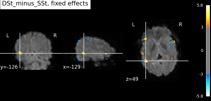
Not unexpectedly, the fixed effects version displays higher peaks than the input runs. Computing fixed effects enhances the signal-to-noise ratio of the resulting brain maps.
Compute fixed effects statistics using preprocessed data of both runs
A more straightforward alternative to fitting run-specific GLMs,
than combining the results with compute_fixed_effects,
is to simply fit the GLM to both runs at once.
Since we can assume that the design matrices of both runs have the same columns, in the same order, we can again reuse the first run’s contrast vector.
/home/runner/work/nilearn/nilearn/examples/04_glm_first_level/plot_two_runs_model.py:183: RuntimeWarning:

[MultiNiftiMasker.fit] Generation of a mask has been requested (imgs != None) while a mask was given at masker creation. Given mask will be used.

\[FirstLevelModel.fit] Computing run 1 out of 2 runs (go take a coffee, a big
one).
\[FirstLevelModel.fit] Performing mask computation.
\[FirstLevelModel.fit] Masking took 1 seconds.
\[FirstLevelModel.fit] Performing GLM computation.
\[FirstLevelModel.fit] GLM took 0 seconds.
\[FirstLevelModel.fit] Computing run 2 out of 2 runs (00 HR 00 MIN 02 SEC
remaining).
\[FirstLevelModel.fit] Performing mask computation.
\[FirstLevelModel.fit] Masking took 1 seconds.
\[FirstLevelModel.fit] Performing GLM computation.
\[FirstLevelModel.fit] GLM took 0 seconds.
\[FirstLevelModel.fit] Computation of 2 runs done in 00 HR 00 MIN 04 SEC.
We can just define the contrast array for one run and assume that the design matrix is the same for the other. However, if we want to be safe, we should define each contrast separately, and provide it as a list.
contrast_val = [
    np.array([[-1, -1, 1, 1]]),  # run 1
    np.array([[-1, -1, 1, 1]]),  # run 2
]

z_map = fmri_glm_multirun.compute_contrast(
    contrast_val,
    output_type="z_score",
)
plot_stat_map(
    z_map,
    bg_img=mean_img_,
    threshold=threshold,
    cut_coords=cut_coords,
    title=f"{contrast_id}, fixed effects",
    vmax=vmax,
)

show()

/home/runner/work/nilearn/nilearn/examples/04_glm_first_level/plot_two_runs_model.py:195: UserWarning:

t contrasts should be of length P=13, but it has length 4. The rest of the contrast was padded with zeros.
You may note that the results are the same as the first fixed effects analysis, but with a lot less code.
Compute a range of contrasts across both runs
It may be useful to investigate a number of contrasts. Therefore, we will move beyond the original contrast of interest and both define and compute several.
Contrast specification
n_columns = design_matrices[0].shape[1]
contrasts = {
    "SStSSp_minus_DStDSp": np.array([[1, 0, 0, -1]]),
    "DStDSp_minus_SStSSp": np.array([[-1, 0, 0, 1]]),
    "DSt_minus_SSt": np.array([[-1, -1, 1, 1]]),
    "DSp_minus_SSp": np.array([[-1, 1, -1, 1]]),
    "DSt_minus_SSt_for_DSp": np.array([[0, -1, 0, 1]]),
    "DSp_minus_SSp_for_DSt": np.array([[0, 0, -1, 1]]),
    "Deactivation": np.array([[-1, -1, -1, -1, 4]]),
    "Effects_of_interest": np.eye(n_columns)[:5, :],  # An F-contrast
}
Next, we compute and plot the statistics for these new contrasts.
print("Computing contrasts...")
for index, (contrast_id, contrast_val) in enumerate(contrasts.items()):
    print(f"  Contrast {index + 1:02g} out of {len(contrasts)}: {contrast_id}")
    # Estimate the contasts.
    z_map = fmri_glm.compute_contrast(contrast_val, output_type="z_score")

    # Write the resulting stat images to file.
    z_image_path = output_dir / f"{contrast_id}_z_map.nii.gz"
    z_map.to_filename(z_image_path)
Computing contrasts...
  Contrast 01 out of 8: SStSSp_minus_DStDSp
/home/runner/work/nilearn/nilearn/examples/04_glm_first_level/plot_two_runs_model.py:242: RuntimeWarning:

The same contrast will be used for all 2 runs. If the design matrices are not the same for all runs, (for example with different column names or column order across runs) you should pass contrast as an expression using the name of the conditions as they appear in the design matrices.

/home/runner/work/nilearn/nilearn/examples/04_glm_first_level/plot_two_runs_model.py:242: UserWarning:

t contrasts should be of length P=13, but it has length 4. The rest of the contrast was padded with zeros.

  Contrast 02 out of 8: DStDSp_minus_SStSSp
  Contrast 03 out of 8: DSt_minus_SSt
  Contrast 04 out of 8: DSp_minus_SSp
  Contrast 05 out of 8: DSt_minus_SSt_for_DSp
  Contrast 06 out of 8: DSp_minus_SSp_for_DSt
  Contrast 07 out of 8: Deactivation
/home/runner/work/nilearn/nilearn/examples/04_glm_first_level/plot_two_runs_model.py:242: UserWarning:

t contrasts should be of length P=13, but it has length 5. The rest of the contrast was padded with zeros.

  Contrast 08 out of 8: Effects_of_interest
/home/runner/work/nilearn/nilearn/examples/04_glm_first_level/plot_two_runs_model.py:242: UserWarning:

Running approximate fixed effects on F statistics.
Generating a report
Since we have already computed the FirstLevelModel and have a number of contrasts, we can quickly create a summary report.
report = fmri_glm_multirun.generate_report(
    contrasts,
    bg_img=mean_img_,
    title="two-runs fMRI model fitting",
)
/home/runner/work/nilearn/nilearn/examples/04_glm_first_level/plot_two_runs_model.py:254: RuntimeWarning:

The same contrast will be used for all 2 runs. If the design matrices are not the same for all runs, (for example with different column names or column order across runs) you should pass contrast as an expression using the name of the conditions as they appear in the design matrices.

/home/runner/work/nilearn/nilearn/examples/04_glm_first_level/plot_two_runs_model.py:254: UserWarning:

t contrasts should be of length P=13, but it has length 4. The rest of the contrast was padded with zeros.

/home/runner/work/nilearn/nilearn/examples/04_glm_first_level/plot_two_runs_model.py:254: UserWarning:

t contrasts should be of length P=13, but it has length 5. The rest of the contrast was padded with zeros.

/home/runner/work/nilearn/nilearn/examples/04_glm_first_level/plot_two_runs_model.py:254: UserWarning:

Running approximate fixed effects on F statistics.

/home/runner/work/nilearn/nilearn/examples/04_glm_first_level/plot_two_runs_model.py:254: UserWarning:

Contrasts will be padded with 9 column(s) of zeros.

/home/runner/work/nilearn/nilearn/examples/04_glm_first_level/plot_two_runs_model.py:254: UserWarning:

Contrasts will be padded with 9 column(s) of zeros.

/home/runner/work/nilearn/nilearn/examples/04_glm_first_level/plot_two_runs_model.py:254: UserWarning:

Contrasts will be padded with 9 column(s) of zeros.

/home/runner/work/nilearn/nilearn/examples/04_glm_first_level/plot_two_runs_model.py:254: UserWarning:

Contrasts will be padded with 9 column(s) of zeros.

/home/runner/work/nilearn/nilearn/examples/04_glm_first_level/plot_two_runs_model.py:254: UserWarning:

Contrasts will be padded with 9 column(s) of zeros.

/home/runner/work/nilearn/nilearn/examples/04_glm_first_level/plot_two_runs_model.py:254: UserWarning:

Contrasts will be padded with 9 column(s) of zeros.

/home/runner/work/nilearn/nilearn/examples/04_glm_first_level/plot_two_runs_model.py:254: UserWarning:

Contrasts will be padded with 8 column(s) of zeros.

/home/runner/work/nilearn/nilearn/examples/04_glm_first_level/plot_two_runs_model.py:254: UserWarning:

Contrasts will be padded with 9 column(s) of zeros.

/home/runner/work/nilearn/nilearn/examples/04_glm_first_level/plot_two_runs_model.py:254: UserWarning:

Contrasts will be padded with 9 column(s) of zeros.

/home/runner/work/nilearn/nilearn/examples/04_glm_first_level/plot_two_runs_model.py:254: UserWarning:

Contrasts will be padded with 9 column(s) of zeros.

/home/runner/work/nilearn/nilearn/examples/04_glm_first_level/plot_two_runs_model.py:254: UserWarning:

Contrasts will be padded with 9 column(s) of zeros.

/home/runner/work/nilearn/nilearn/examples/04_glm_first_level/plot_two_runs_model.py:254: UserWarning:

Contrasts will be padded with 9 column(s) of zeros.

/home/runner/work/nilearn/nilearn/examples/04_glm_first_level/plot_two_runs_model.py:254: UserWarning:

Contrasts will be padded with 9 column(s) of zeros.

/home/runner/work/nilearn/nilearn/examples/04_glm_first_level/plot_two_runs_model.py:254: UserWarning:

Contrasts will be padded with 8 column(s) of zeros.
Note
The generated report can be:
displayed in a Notebook,
opened in a browser using the
.open_in_browser()method,or saved to a file using the
.save_as_html(output_filepath)method.
two-runs fMRI model fitting Implement the General Linear Model for single run :term:`fMRI` data.
Description
Data were analyzed using Nilearn (version= 0.14.1; RRID:SCR_001362).
At the subject level, a mass univariate analysis was performed with a linear regression at each voxel of the brain, using generalized least squares with a global ar1 noise model to account for temporal auto-correlation and a cosine drift model (high pass filter=0.01 Hz).
Input images were smoothed with gaussian kernel (full-width at half maximum=5 mm).
Model details
| Value | |
|---|---|
| Parameter | |
| drift_model | cosine |
| high_pass (Hertz) | 0.01 |
| hrf_model | glover |
| noise_model | ar1 |
| signal_scaling | 0 |
| slice_time_ref | 0.0 |
| smoothing_fwhm (mm) | 5 |
| standardize | False |
You can cycle through the different runs using your left and right arrow keys.


.")
.")
.")
.")
.")
.")
.")
.")


Mask

The mask includes 28008 voxels (22.8 %) of the image.
Statistical Maps
SStSSp_minus_DStDSp

Cluster Table
| Height control | fpr |
|---|---|
| α | 0.001 |
| Threshold (computed) | 3.09 |
| Cluster size threshold (voxels) | 0 |
| Minimum distance (mm) | 8.0 |
| Cluster ID | X | Y | Z | Peak Stat | Cluster Size (mm3) |
|---|---|---|---|---|---|
| 1 | -135.0 | -138.0 | 40.0 | 5.42 | 828 |
| 2 | -111.0 | -57.0 | 92.0 | 5.14 | 432 |
| 3 | -111.0 | -27.0 | 52.0 | 4.85 | 324 |
| 4 | -126.0 | -150.0 | 80.0 | 4.67 | 504 |
| 4a | -126.0 | -153.0 | 64.0 | 4.05 | |
| 5 | -141.0 | -114.0 | 40.0 | 4.61 | 468 |
| 6 | -132.0 | -105.0 | 88.0 | 4.46 | 144 |
| 7 | -138.0 | -54.0 | 56.0 | 4.37 | 504 |
| 8 | -135.0 | -138.0 | 80.0 | 4.25 | 1152 |
| 8a | -144.0 | -120.0 | 76.0 | 3.65 | |
| 8b | -138.0 | -126.0 | 88.0 | 3.46 | |
| 9 | -102.0 | -90.0 | 104.0 | 4.23 | 144 |
| 10 | -39.0 | -102.0 | 60.0 | 4.22 | 108 |
| 11 | -120.0 | -69.0 | 96.0 | 4.15 | 180 |
| 12 | -132.0 | -39.0 | 52.0 | 4.10 | 36 |
| 13 | -120.0 | -96.0 | 20.0 | 4.01 | 108 |
| 14 | -99.0 | -144.0 | 36.0 | 3.93 | 72 |
| 15 | -90.0 | -117.0 | 92.0 | 3.86 | 36 |
| 16 | -81.0 | -30.0 | 76.0 | 3.85 | 324 |
| 16a | -90.0 | -33.0 | 76.0 | 3.27 | |
| 17 | -93.0 | -87.0 | 80.0 | 3.83 | 72 |
| 18 | -75.0 | -30.0 | 56.0 | 3.79 | 144 |
| 19 | -135.0 | -42.0 | 56.0 | 3.72 | 72 |
| 20 | -135.0 | -63.0 | 76.0 | 3.71 | 108 |
| 21 | -51.0 | -69.0 | 48.0 | 3.71 | 36 |
| 22 | -111.0 | -72.0 | 84.0 | 3.70 | 72 |
| 23 | -132.0 | -66.0 | 36.0 | 3.69 | 36 |
| 24 | -102.0 | -105.0 | 112.0 | 3.68 | 36 |
| 25 | -135.0 | -141.0 | 56.0 | 3.68 | 72 |
| 26 | -141.0 | -87.0 | 60.0 | 3.67 | 252 |
| 27 | -141.0 | -63.0 | 48.0 | 3.66 | 36 |
| 28 | -81.0 | -111.0 | 8.0 | 3.64 | 36 |
| 29 | -132.0 | -129.0 | 92.0 | 3.63 | 108 |
| 30 | -111.0 | -114.0 | 32.0 | 3.62 | 72 |
| 31 | -57.0 | -102.0 | 88.0 | 3.62 | 36 |
| 32 | -135.0 | -42.0 | 48.0 | 3.61 | 36 |
| 33 | -126.0 | -39.0 | 48.0 | 3.60 | 72 |
| 34 | -54.0 | -141.0 | 88.0 | 3.55 | 72 |
| 35 | -81.0 | -108.0 | 64.0 | 3.55 | 36 |
| 36 | -78.0 | -63.0 | 32.0 | 3.55 | 144 |
| 37 | -144.0 | -93.0 | 64.0 | 3.53 | 72 |
| 38 | -114.0 | -150.0 | 80.0 | 3.52 | 216 |
| 39 | -144.0 | -129.0 | 68.0 | 3.50 | 36 |
| 40 | -144.0 | -78.0 | 72.0 | 3.50 | 36 |
| 41 | -135.0 | -90.0 | 88.0 | 3.50 | 36 |
| 42 | -144.0 | -111.0 | 80.0 | 3.48 | 36 |
| 43 | -72.0 | -126.0 | 56.0 | 3.47 | 36 |
| 44 | -93.0 | -60.0 | 100.0 | 3.44 | 36 |
| 45 | -90.0 | -18.0 | 60.0 | 3.42 | 72 |
| 46 | -87.0 | -93.0 | 112.0 | 3.41 | 36 |
| 47 | -135.0 | -57.0 | 72.0 | 3.39 | 36 |
| 48 | -120.0 | -30.0 | 44.0 | 3.38 | 36 |
| 49 | -129.0 | -147.0 | 72.0 | 3.35 | 36 |
| 50 | -123.0 | -45.0 | 48.0 | 3.34 | 36 |
| 51 | -129.0 | -87.0 | 44.0 | 3.34 | 36 |
| 52 | -93.0 | -84.0 | 112.0 | 3.34 | 72 |
| 53 | -66.0 | -150.0 | 12.0 | 3.34 | 36 |
| 54 | -123.0 | -45.0 | 80.0 | 3.34 | 36 |
| 55 | -114.0 | -33.0 | 76.0 | 3.31 | 72 |
| 56 | -51.0 | -78.0 | 28.0 | 3.31 | 72 |
| 57 | -123.0 | -102.0 | 100.0 | 3.30 | 36 |
| 58 | -117.0 | -87.0 | 92.0 | 3.30 | 36 |
| 59 | -51.0 | -87.0 | 96.0 | 3.30 | 36 |
| 60 | -144.0 | -102.0 | 76.0 | 3.29 | 36 |
| 61 | -129.0 | -90.0 | 80.0 | 3.28 | 36 |
| 62 | -138.0 | -51.0 | 44.0 | 3.27 | 36 |
| 63 | -123.0 | -108.0 | 84.0 | 3.26 | 36 |
| 64 | -132.0 | -69.0 | 32.0 | 3.26 | 36 |
| 65 | -129.0 | -60.0 | 84.0 | 3.26 | 36 |
| 66 | -51.0 | -75.0 | 44.0 | 3.26 | 72 |
| 67 | -90.0 | -141.0 | 36.0 | 3.26 | 36 |
| 68 | -90.0 | -87.0 | 108.0 | 3.26 | 36 |
| 69 | -114.0 | -27.0 | 56.0 | 3.25 | 36 |
| 70 | -138.0 | -141.0 | 60.0 | 3.23 | 36 |
| 71 | -57.0 | -102.0 | 72.0 | 3.23 | 36 |
| 72 | -84.0 | -33.0 | 72.0 | 3.23 | 36 |
| 73 | -75.0 | -126.0 | 60.0 | 3.22 | 36 |
| 74 | -78.0 | -69.0 | 92.0 | 3.22 | 36 |
| 75 | -141.0 | -60.0 | 60.0 | 3.21 | 36 |
| 76 | -141.0 | -135.0 | 72.0 | 3.21 | 36 |
| 77 | -93.0 | -78.0 | 76.0 | 3.21 | 108 |
| 78 | -84.0 | -63.0 | 36.0 | 3.16 | 36 |
| 79 | -111.0 | -48.0 | 92.0 | 3.14 | 36 |
| 80 | -117.0 | -147.0 | 76.0 | 3.14 | 36 |
| 81 | -87.0 | -111.0 | 88.0 | 3.14 | 36 |
| 82 | -120.0 | -81.0 | 100.0 | 3.13 | 36 |
| 83 | -111.0 | -30.0 | 76.0 | 3.13 | 36 |
| 84 | -117.0 | -24.0 | 56.0 | 3.13 | 36 |
| 85 | -108.0 | -138.0 | 40.0 | 3.12 | 36 |
| 86 | -108.0 | -30.0 | 72.0 | 3.12 | 36 |
| 87 | -120.0 | -42.0 | 56.0 | 3.12 | 36 |
| 88 | -87.0 | -120.0 | 92.0 | 3.11 | 36 |
| 89 | -126.0 | -33.0 | 48.0 | 3.10 | 36 |
| 90 | -87.0 | -54.0 | 48.0 | 3.10 | 36 |
| 91 | -54.0 | -90.0 | 92.0 | 3.10 | 36 |
| 92 | -129.0 | -72.0 | 92.0 | 3.09 | 36 |
| 93 | -132.0 | -144.0 | 80.0 | 3.09 | 36 |
DStDSp_minus_SStSSp

Cluster Table
| Height control | fpr |
|---|---|
| α | 0.001 |
| Threshold (computed) | 3.09 |
| Cluster size threshold (voxels) | 0 |
| Minimum distance (mm) | 8.0 |
| Cluster ID | X | Y | Z | Peak Stat | Cluster Size (mm3) |
|---|---|---|---|---|---|
| 1 | -72.0 | -147.0 | 8.0 | 5.53 | 504 |
| 1a | -69.0 | -135.0 | 8.0 | 3.57 | |
| 2 | -96.0 | -147.0 | 4.0 | 5.28 | 828 |
| 2a | -99.0 | -144.0 | 12.0 | 3.99 | |
| 3 | -60.0 | -126.0 | 4.0 | 5.20 | 216 |
| 4 | -99.0 | -75.0 | 108.0 | 4.98 | 396 |
| 5 | -132.0 | -129.0 | 52.0 | 4.95 | 828 |
| 6 | -105.0 | -108.0 | 92.0 | 4.56 | 36 |
| 7 | -129.0 | -60.0 | 48.0 | 4.55 | 396 |
| 8 | -42.0 | -66.0 | 48.0 | 4.51 | 72 |
| 9 | -54.0 | -111.0 | 48.0 | 4.49 | 144 |
| 10 | -33.0 | -66.0 | 44.0 | 4.42 | 36 |
| 11 | -39.0 | -84.0 | 88.0 | 4.21 | 72 |
| 12 | -45.0 | -63.0 | 80.0 | 4.10 | 36 |
| 13 | -51.0 | -42.0 | 24.0 | 4.10 | 72 |
| 14 | -87.0 | -42.0 | 88.0 | 4.09 | 72 |
| 15 | -33.0 | -114.0 | 68.0 | 4.05 | 72 |
| 16 | -51.0 | -114.0 | 36.0 | 4.03 | 108 |
| 17 | -75.0 | -150.0 | 8.0 | 4.02 | 36 |
| 18 | -45.0 | -66.0 | 84.0 | 3.94 | 72 |
| 19 | -72.0 | -147.0 | 84.0 | 3.91 | 36 |
| 20 | -36.0 | -90.0 | 72.0 | 3.91 | 36 |
| 21 | -138.0 | -99.0 | 44.0 | 3.87 | 72 |
| 22 | -99.0 | -141.0 | 20.0 | 3.85 | 36 |
| 23 | -138.0 | -105.0 | 48.0 | 3.83 | 144 |
| 24 | -126.0 | -75.0 | 72.0 | 3.82 | 72 |
| 25 | -51.0 | -108.0 | 88.0 | 3.81 | 72 |
| 26 | -108.0 | -138.0 | 0.0 | 3.80 | 108 |
| 27 | -75.0 | -63.0 | 60.0 | 3.79 | 108 |
| 28 | -51.0 | -102.0 | 96.0 | 3.76 | 72 |
| 29 | -135.0 | -78.0 | 68.0 | 3.76 | 144 |
| 30 | -69.0 | -72.0 | 56.0 | 3.75 | 72 |
| 31 | -39.0 | -78.0 | 48.0 | 3.75 | 396 |
| 32 | -51.0 | -117.0 | 48.0 | 3.71 | 72 |
| 33 | -45.0 | -54.0 | 64.0 | 3.65 | 72 |
| 34 | -48.0 | -102.0 | 36.0 | 3.64 | 216 |
| 35 | -57.0 | -96.0 | 48.0 | 3.63 | 36 |
| 36 | -39.0 | -87.0 | 76.0 | 3.61 | 36 |
| 37 | -39.0 | -78.0 | 84.0 | 3.60 | 36 |
| 38 | -48.0 | -66.0 | 80.0 | 3.59 | 36 |
| 39 | -138.0 | -108.0 | 76.0 | 3.58 | 36 |
| 40 | -96.0 | -159.0 | 60.0 | 3.58 | 36 |
| 41 | -126.0 | -141.0 | 56.0 | 3.51 | 36 |
| 42 | -48.0 | -114.0 | 64.0 | 3.47 | 36 |
| 43 | -117.0 | -123.0 | 48.0 | 3.44 | 72 |
| 44 | -36.0 | -93.0 | 76.0 | 3.42 | 108 |
| 45 | -96.0 | -99.0 | 104.0 | 3.39 | 72 |
| 46 | -48.0 | -123.0 | 40.0 | 3.38 | 36 |
| 47 | -48.0 | -108.0 | 32.0 | 3.35 | 36 |
| 48 | -69.0 | -87.0 | 96.0 | 3.33 | 72 |
| 49 | -48.0 | -156.0 | 48.0 | 3.22 | 36 |
| 50 | -69.0 | -129.0 | 80.0 | 3.22 | 36 |
| 51 | -81.0 | -69.0 | 64.0 | 3.22 | 36 |
| 52 | -66.0 | -135.0 | 20.0 | 3.19 | 36 |
| 53 | -39.0 | -93.0 | 72.0 | 3.19 | 36 |
| 54 | -63.0 | -108.0 | 68.0 | 3.19 | 36 |
| 55 | -102.0 | -129.0 | 80.0 | 3.18 | 36 |
| 56 | -123.0 | -141.0 | 44.0 | 3.15 | 36 |
| 57 | -48.0 | -51.0 | 64.0 | 3.14 | 36 |
| 58 | -42.0 | -72.0 | 56.0 | 3.13 | 36 |
| 59 | -135.0 | -57.0 | 20.0 | 3.10 | 36 |
| 60 | -75.0 | -141.0 | 12.0 | 3.10 | 36 |
| 61 | -36.0 | -126.0 | 76.0 | 3.10 | 36 |
| 62 | -60.0 | -66.0 | 68.0 | 3.10 | 36 |
DSt_minus_SSt

Cluster Table
| Height control | fpr |
|---|---|
| α | 0.001 |
| Threshold (computed) | 3.09 |
| Cluster size threshold (voxels) | 0 |
| Minimum distance (mm) | 8.0 |
| Cluster ID | X | Y | Z | Peak Stat | Cluster Size (mm3) |
|---|---|---|---|---|---|
| 1 | -129.0 | -129.0 | 48.0 | 5.30 | 576 |
| 2 | -129.0 | -60.0 | 48.0 | 4.48 | 144 |
| 3 | -99.0 | -75.0 | 108.0 | 4.43 | 288 |
| 4 | -51.0 | -42.0 | 24.0 | 4.41 | 108 |
| 5 | -42.0 | -66.0 | 48.0 | 4.26 | 72 |
| 6 | -33.0 | -66.0 | 44.0 | 4.24 | 36 |
| 7 | -135.0 | -57.0 | 20.0 | 4.19 | 36 |
| 8 | -72.0 | -147.0 | 8.0 | 4.03 | 324 |
| 8a | -69.0 | -135.0 | 8.0 | 3.64 | |
| 9 | -84.0 | -81.0 | 44.0 | 4.03 | 72 |
| 10 | -102.0 | -138.0 | 12.0 | 4.00 | 144 |
| 11 | -138.0 | -105.0 | 48.0 | 3.99 | 108 |
| 12 | -51.0 | -114.0 | 36.0 | 3.91 | 108 |
| 13 | -96.0 | -147.0 | 4.0 | 3.70 | 72 |
| 14 | -45.0 | -69.0 | 84.0 | 3.67 | 108 |
| 15 | -120.0 | -78.0 | 44.0 | 3.54 | 36 |
| 16 | -42.0 | -60.0 | 24.0 | 3.54 | 36 |
| 17 | -138.0 | -99.0 | 44.0 | 3.36 | 36 |
| 18 | -45.0 | -57.0 | 16.0 | 3.36 | 36 |
| 19 | -114.0 | -75.0 | 60.0 | 3.35 | 36 |
| 20 | -117.0 | -60.0 | 64.0 | 3.33 | 36 |
| 21 | -78.0 | -138.0 | 16.0 | 3.32 | 36 |
| 22 | -33.0 | -114.0 | 68.0 | 3.32 | 36 |
| 23 | -132.0 | -63.0 | 16.0 | 3.31 | 72 |
| 24 | -81.0 | -84.0 | 44.0 | 3.29 | 72 |
| 25 | -36.0 | -93.0 | 80.0 | 3.26 | 36 |
| 26 | -48.0 | -54.0 | 16.0 | 3.25 | 36 |
| 27 | -78.0 | -60.0 | 60.0 | 3.20 | 36 |
| 28 | -105.0 | -135.0 | 0.0 | 3.19 | 36 |
| 29 | -141.0 | -48.0 | 32.0 | 3.19 | 36 |
| 30 | -51.0 | -117.0 | 48.0 | 3.17 | 36 |
| 31 | -96.0 | -144.0 | 12.0 | 3.17 | 72 |
| 32 | -48.0 | -120.0 | 48.0 | 3.17 | 36 |
| 33 | -36.0 | -90.0 | 44.0 | 3.17 | 36 |
| 34 | -135.0 | -78.0 | 68.0 | 3.13 | 36 |
| 35 | -54.0 | -108.0 | 40.0 | 3.11 | 36 |
| 36 | -126.0 | -69.0 | 28.0 | 3.11 | 36 |
DSp_minus_SSp

Cluster Table
| Height control | fpr |
|---|---|
| α | 0.001 |
| Threshold (computed) | 3.09 |
| Cluster size threshold (voxels) | 0 |
| Minimum distance (mm) | 8.0 |
| Cluster ID | X | Y | Z | Peak Stat | Cluster Size (mm3) |
|---|---|---|---|---|---|
| 1 | -54.0 | -111.0 | 52.0 | 4.92 | 396 |
| 2 | -60.0 | -126.0 | 4.0 | 4.84 | 252 |
| 3 | -105.0 | -108.0 | 92.0 | 4.60 | 72 |
| 4 | -48.0 | -114.0 | 64.0 | 4.47 | 144 |
| 5 | -63.0 | -108.0 | 68.0 | 4.12 | 108 |
| 6 | -48.0 | -102.0 | 32.0 | 4.03 | 216 |
| 7 | -48.0 | -123.0 | 40.0 | 3.97 | 72 |
| 8 | -87.0 | -42.0 | 88.0 | 3.95 | 72 |
| 9 | -105.0 | -141.0 | 4.0 | 3.93 | 108 |
| 10 | -72.0 | -147.0 | 8.0 | 3.81 | 108 |
| 11 | -72.0 | -87.0 | 96.0 | 3.74 | 72 |
| 12 | -96.0 | -147.0 | 4.0 | 3.73 | 108 |
| 13 | -102.0 | -135.0 | 28.0 | 3.72 | 108 |
| 14 | -45.0 | -63.0 | 80.0 | 3.72 | 72 |
| 15 | -36.0 | -96.0 | 56.0 | 3.70 | 72 |
| 16 | -135.0 | -108.0 | 76.0 | 3.68 | 180 |
| 17 | -126.0 | -111.0 | 68.0 | 3.63 | 36 |
| 18 | -45.0 | -84.0 | 48.0 | 3.61 | 72 |
| 19 | -54.0 | -96.0 | 44.0 | 3.57 | 108 |
| 20 | -120.0 | -123.0 | 48.0 | 3.57 | 36 |
| 21 | -96.0 | -102.0 | 104.0 | 3.56 | 108 |
| 22 | -39.0 | -114.0 | 56.0 | 3.54 | 216 |
| 23 | -60.0 | -87.0 | 100.0 | 3.51 | 72 |
| 24 | -114.0 | -87.0 | 36.0 | 3.50 | 36 |
| 25 | -42.0 | -111.0 | 36.0 | 3.45 | 108 |
| 26 | -96.0 | -159.0 | 60.0 | 3.41 | 36 |
| 27 | -45.0 | -105.0 | 56.0 | 3.38 | 108 |
| 28 | -66.0 | -144.0 | 56.0 | 3.36 | 72 |
| 29 | -114.0 | -153.0 | 36.0 | 3.32 | 36 |
| 30 | -78.0 | -99.0 | 56.0 | 3.32 | 36 |
| 31 | -69.0 | -69.0 | 56.0 | 3.32 | 72 |
| 32 | -39.0 | -84.0 | 88.0 | 3.30 | 36 |
| 33 | -102.0 | -117.0 | 72.0 | 3.30 | 36 |
| 34 | -129.0 | -60.0 | 52.0 | 3.28 | 36 |
| 35 | -126.0 | -117.0 | 32.0 | 3.26 | 36 |
| 36 | -132.0 | -123.0 | 48.0 | 3.25 | 36 |
| 37 | -39.0 | -81.0 | 52.0 | 3.25 | 36 |
| 38 | -102.0 | -144.0 | 8.0 | 3.23 | 36 |
| 39 | -81.0 | -102.0 | 36.0 | 3.21 | 36 |
| 40 | -78.0 | -165.0 | 44.0 | 3.21 | 36 |
| 41 | -60.0 | -138.0 | 52.0 | 3.19 | 36 |
| 42 | -96.0 | -162.0 | 56.0 | 3.18 | 36 |
| 43 | -51.0 | -78.0 | 92.0 | 3.17 | 36 |
| 44 | -45.0 | -66.0 | 56.0 | 3.15 | 36 |
| 45 | -48.0 | -63.0 | 56.0 | 3.14 | 36 |
| 46 | -126.0 | -60.0 | 48.0 | 3.13 | 36 |
| 47 | -45.0 | -57.0 | 64.0 | 3.13 | 36 |
| 48 | -66.0 | -129.0 | 4.0 | 3.12 | 36 |
| 49 | -75.0 | -150.0 | 8.0 | 3.12 | 36 |
DSt_minus_SSt_for_DSp

Cluster Table
| Height control | fpr |
|---|---|
| α | 0.001 |
| Threshold (computed) | 3.09 |
| Cluster size threshold (voxels) | 0 |
| Minimum distance (mm) | 8.0 |
| Cluster ID | X | Y | Z | Peak Stat | Cluster Size (mm3) |
|---|---|---|---|---|---|
| 1 | -102.0 | -129.0 | 48.0 | 4.46 | 36 |
| 2 | -105.0 | -135.0 | 0.0 | 4.28 | 108 |
| 3 | -129.0 | -126.0 | 48.0 | 3.81 | 144 |
| 4 | -84.0 | -81.0 | 44.0 | 3.76 | 36 |
| 5 | -111.0 | -66.0 | 68.0 | 3.35 | 36 |
| 6 | -66.0 | -168.0 | 48.0 | 3.34 | 36 |
| 7 | -66.0 | -69.0 | 96.0 | 3.23 | 36 |
| 8 | -69.0 | -69.0 | 64.0 | 3.16 | 36 |
| 9 | -75.0 | -108.0 | 12.0 | 3.14 | 36 |
DSp_minus_SSp_for_DSt

Cluster Table
| Height control | fpr |
|---|---|
| α | 0.001 |
| Threshold (computed) | 3.09 |
| Cluster size threshold (voxels) | 0 |
| Minimum distance (mm) | 8.0 |
| Cluster ID | X | Y | Z | Peak Stat | Cluster Size (mm3) |
|---|---|---|---|---|---|
| 1 | -78.0 | -60.0 | 40.0 | 3.68 | 36 |
| 2 | -72.0 | -87.0 | 96.0 | 3.68 | 36 |
| 3 | -108.0 | -69.0 | 76.0 | 3.60 | 36 |
| 4 | -102.0 | -117.0 | 108.0 | 3.58 | 72 |
| 5 | -66.0 | -99.0 | 92.0 | 3.57 | 72 |
| 6 | -93.0 | -153.0 | 20.0 | 3.49 | 72 |
| 7 | -75.0 | -90.0 | 100.0 | 3.46 | 36 |
| 8 | -108.0 | -135.0 | 0.0 | 3.38 | 36 |
| 9 | -132.0 | -111.0 | 72.0 | 3.36 | 36 |
| 10 | -114.0 | -132.0 | 48.0 | 3.34 | 36 |
| 11 | -99.0 | -99.0 | 104.0 | 3.31 | 72 |
| 12 | -51.0 | -123.0 | 40.0 | 3.26 | 36 |
| 13 | -81.0 | -129.0 | 112.0 | 3.25 | 36 |
| 14 | -60.0 | -126.0 | 4.0 | 3.21 | 36 |
| 15 | -63.0 | -102.0 | 108.0 | 3.20 | 36 |
| 16 | -63.0 | -81.0 | 32.0 | 3.19 | 36 |
| 17 | -117.0 | -126.0 | 20.0 | 3.16 | 36 |
| 18 | -120.0 | -42.0 | 24.0 | 3.14 | 36 |
| 19 | -72.0 | -69.0 | 80.0 | 3.12 | 36 |
| 20 | -114.0 | -66.0 | 68.0 | 3.11 | 36 |
| 21 | -102.0 | -159.0 | 44.0 | 3.10 | 36 |
Deactivation

Cluster Table
| Height control | fpr |
|---|---|
| α | 0.001 |
| Threshold (computed) | 3.09 |
| Cluster size threshold (voxels) | 0 |
| Minimum distance (mm) | 8.0 |
| Cluster ID | X | Y | Z | Peak Stat | Cluster Size (mm3) |
|---|---|---|---|---|---|
| 1 | -48.0 | -93.0 | 56.0 | 5.97 | 5652 |
| 1a | -39.0 | -93.0 | 64.0 | 5.64 | |
| 1b | -39.0 | -114.0 | 60.0 | 5.27 | |
| 1c | -51.0 | -96.0 | 64.0 | 5.24 | |
| 2 | -51.0 | -60.0 | 56.0 | 5.70 | 3204 |
| 3 | -138.0 | -81.0 | 60.0 | 5.05 | 576 |
| 3a | -129.0 | -81.0 | 64.0 | 3.61 | |
| 4 | -120.0 | -114.0 | 56.0 | 5.00 | 4284 |
| 4a | -135.0 | -123.0 | 56.0 | 4.76 | |
| 4b | -126.0 | -108.0 | 60.0 | 4.71 | |
| 4c | -129.0 | -129.0 | 52.0 | 4.63 | |
| 5 | -102.0 | -75.0 | 104.0 | 4.90 | 288 |
| 6 | -90.0 | -69.0 | 100.0 | 4.61 | 324 |
| 6a | -90.0 | -72.0 | 92.0 | 4.34 | |
| 7 | -51.0 | -117.0 | 60.0 | 4.52 | 576 |
| 8 | -57.0 | -78.0 | 96.0 | 4.41 | 756 |
| 8a | -54.0 | -75.0 | 88.0 | 4.41 | |
| 9 | -54.0 | -63.0 | 76.0 | 4.18 | 396 |
| 9a | -45.0 | -60.0 | 76.0 | 3.31 | |
| 10 | -132.0 | -60.0 | 48.0 | 4.17 | 180 |
| 11 | -36.0 | -111.0 | 72.0 | 4.06 | 108 |
| 12 | -48.0 | -114.0 | 68.0 | 4.03 | 108 |
| 13 | -90.0 | -81.0 | 108.0 | 3.92 | 72 |
| 14 | -111.0 | -117.0 | 80.0 | 3.85 | 36 |
| 15 | -138.0 | -96.0 | 44.0 | 3.80 | 108 |
| 16 | -120.0 | -66.0 | 52.0 | 3.71 | 180 |
| 17 | -54.0 | -69.0 | 72.0 | 3.53 | 36 |
| 18 | -90.0 | -75.0 | 104.0 | 3.49 | 36 |
| 19 | -45.0 | -66.0 | 80.0 | 3.46 | 36 |
| 20 | -45.0 | -63.0 | 44.0 | 3.44 | 36 |
| 21 | -87.0 | -93.0 | 76.0 | 3.25 | 36 |
| 22 | -45.0 | -66.0 | 40.0 | 3.21 | 36 |
| 23 | -39.0 | -87.0 | 84.0 | 3.21 | 72 |
| 24 | -42.0 | -108.0 | 56.0 | 3.19 | 36 |
Effects_of_interest

Cluster Table
| Height control | fpr |
|---|---|
| α | 0.001 |
| Threshold (computed) | 3.09 |
| Cluster size threshold (voxels) | 0 |
| Minimum distance (mm) | 8.0 |
| Cluster ID | X | Y | Z | Peak Stat | Cluster Size (mm3) |
|---|---|---|---|---|---|
| 1 | -33.0 | -111.0 | 56.0 | 16.12 | 50760 |
| 1a | -36.0 | -99.0 | 56.0 | 14.50 | |
| 1b | -45.0 | -75.0 | 56.0 | 14.22 | |
| 1c | -45.0 | -99.0 | 64.0 | 13.56 | |
| 2 | -141.0 | -105.0 | 48.0 | 13.82 | 27684 |
| 2a | -138.0 | -96.0 | 48.0 | 13.76 | |
| 2b | -141.0 | -117.0 | 48.0 | 13.49 | |
| 2c | -138.0 | -111.0 | 56.0 | 13.06 | |
| 3 | -93.0 | -147.0 | 4.0 | 8.75 | 5868 |
| 3a | -108.0 | -141.0 | 0.0 | 7.89 | |
| 3b | -99.0 | -141.0 | 20.0 | 7.05 | |
| 3c | -102.0 | -144.0 | 12.0 | 6.98 | |
| 4 | -87.0 | -111.0 | 88.0 | 8.40 | 34092 |
| 4a | -90.0 | -147.0 | 88.0 | 8.08 | |
| 4b | -96.0 | -138.0 | 104.0 | 7.71 | |
| 4c | -84.0 | -138.0 | 100.0 | 7.53 | |
| 5 | -96.0 | -60.0 | 72.0 | 7.80 | 8964 |
| 5a | -96.0 | -57.0 | 80.0 | 6.92 | |
| 5b | -102.0 | -33.0 | 56.0 | 6.82 | |
| 5c | -96.0 | -69.0 | 80.0 | 6.81 | |
| 6 | -57.0 | -78.0 | 16.0 | 7.75 | 1512 |
| 6a | -51.0 | -78.0 | 28.0 | 3.92 | |
| 7 | -75.0 | -57.0 | 76.0 | 7.68 | 2052 |
| 7a | -69.0 | -66.0 | 88.0 | 4.06 | |
| 7b | -75.0 | -51.0 | 92.0 | 3.62 | |
| 8 | -54.0 | -75.0 | 88.0 | 7.39 | 2664 |
| 8a | -63.0 | -69.0 | 96.0 | 5.13 | |
| 9 | -138.0 | -78.0 | 64.0 | 7.31 | 1476 |
| 9a | -141.0 | -87.0 | 56.0 | 4.45 | |
| 10 | -117.0 | -87.0 | 104.0 | 7.23 | 1908 |
| 10a | -111.0 | -93.0 | 108.0 | 4.96 | |
| 10b | -102.0 | -90.0 | 104.0 | 3.93 | |
| 11 | -72.0 | -147.0 | 8.0 | 7.00 | 2196 |
| 11a | -72.0 | -156.0 | 20.0 | 6.19 | |
| 11b | -66.0 | -147.0 | 20.0 | 5.56 | |
| 12 | -129.0 | -60.0 | 48.0 | 6.92 | 972 |
| 12a | -120.0 | -60.0 | 56.0 | 5.80 | |
| 13 | -102.0 | -75.0 | 104.0 | 6.69 | 360 |
| 14 | -69.0 | -108.0 | 112.0 | 6.47 | 1152 |
| 15 | -111.0 | -117.0 | 32.0 | 6.22 | 936 |
| 15a | -111.0 | -126.0 | 36.0 | 5.54 | |
| 16 | -90.0 | -114.0 | 112.0 | 6.09 | 612 |
| 17 | -120.0 | -132.0 | 24.0 | 5.98 | 576 |
| 18 | -123.0 | -84.0 | 32.0 | 5.57 | 72 |
| 19 | -114.0 | -123.0 | 104.0 | 5.43 | 1836 |
| 19a | -123.0 | -129.0 | 104.0 | 4.39 | |
| 20 | -45.0 | -138.0 | 72.0 | 5.41 | 2916 |
| 20a | -51.0 | -138.0 | 80.0 | 5.39 | |
| 20b | -51.0 | -141.0 | 88.0 | 5.36 | |
| 20c | -51.0 | -150.0 | 72.0 | 4.82 | |
| 21 | -129.0 | -54.0 | 60.0 | 5.37 | 1080 |
| 21a | -138.0 | -57.0 | 64.0 | 4.92 | |
| 22 | -93.0 | -60.0 | 100.0 | 5.36 | 144 |
| 23 | -72.0 | -78.0 | 96.0 | 5.35 | 1404 |
| 23a | -81.0 | -84.0 | 104.0 | 4.55 | |
| 24 | -132.0 | -102.0 | 96.0 | 5.31 | 288 |
| 25 | -57.0 | -111.0 | 12.0 | 5.21 | 540 |
| 25a | -48.0 | -117.0 | 12.0 | 3.66 | |
| 26 | -48.0 | -117.0 | 28.0 | 5.18 | 576 |
| 27 | -90.0 | -96.0 | 112.0 | 5.14 | 684 |
| 27a | -93.0 | -81.0 | 112.0 | 4.18 | |
| 28 | -60.0 | -111.0 | 36.0 | 5.09 | 1404 |
| 28a | -63.0 | -114.0 | 28.0 | 4.23 | |
| 28b | -69.0 | -99.0 | 36.0 | 4.04 | |
| 29 | -87.0 | -36.0 | 48.0 | 5.07 | 720 |
| 30 | -51.0 | -135.0 | 16.0 | 5.03 | 504 |
| 31 | -78.0 | -69.0 | 32.0 | 5.03 | 108 |
| 32 | -123.0 | -117.0 | 32.0 | 5.01 | 144 |
| 33 | -66.0 | -126.0 | 108.0 | 4.99 | 288 |
| 34 | -51.0 | -42.0 | 24.0 | 4.94 | 144 |
| 35 | -123.0 | -108.0 | 80.0 | 4.94 | 648 |
| 35a | -135.0 | -105.0 | 88.0 | 4.91 | |
| 36 | -48.0 | -102.0 | 96.0 | 4.86 | 72 |
| 37 | -69.0 | -84.0 | 24.0 | 4.82 | 108 |
| 38 | -102.0 | -120.0 | 28.0 | 4.76 | 144 |
| 39 | -126.0 | -141.0 | 12.0 | 4.66 | 180 |
| 40 | -63.0 | -54.0 | 92.0 | 4.64 | 36 |
| 41 | -132.0 | -69.0 | 40.0 | 4.62 | 36 |
| 42 | -66.0 | -54.0 | 24.0 | 4.62 | 36 |
| 43 | -51.0 | -42.0 | 64.0 | 4.60 | 36 |
| 44 | -78.0 | -84.0 | 24.0 | 4.60 | 108 |
| 45 | -135.0 | -144.0 | 56.0 | 4.60 | 252 |
| 45a | -138.0 | -141.0 | 68.0 | 3.18 | |
| 46 | -75.0 | -114.0 | 116.0 | 4.60 | 72 |
| 47 | -57.0 | -141.0 | 28.0 | 4.58 | 432 |
| 48 | -123.0 | -102.0 | 64.0 | 4.53 | 72 |
| 49 | -123.0 | -60.0 | 32.0 | 4.50 | 144 |
| 50 | -87.0 | -153.0 | 36.0 | 4.44 | 36 |
| 51 | -144.0 | -102.0 | 60.0 | 4.40 | 36 |
| 52 | -60.0 | -159.0 | 40.0 | 4.39 | 216 |
| 53 | -57.0 | -54.0 | 88.0 | 4.38 | 288 |
| 54 | -78.0 | -126.0 | 0.0 | 4.38 | 324 |
| 55 | -69.0 | -63.0 | 44.0 | 4.37 | 180 |
| 56 | -57.0 | -93.0 | 88.0 | 4.36 | 684 |
| 57 | -132.0 | -69.0 | 32.0 | 4.35 | 72 |
| 58 | -60.0 | -126.0 | 4.0 | 4.32 | 36 |
| 59 | -78.0 | -63.0 | 64.0 | 4.30 | 180 |
| 60 | -135.0 | -93.0 | 88.0 | 4.28 | 144 |
| 61 | -102.0 | -57.0 | 100.0 | 4.25 | 36 |
| 62 | -114.0 | -150.0 | 28.0 | 4.23 | 252 |
| 63 | -138.0 | -78.0 | 40.0 | 4.18 | 72 |
| 64 | -51.0 | -108.0 | 28.0 | 4.17 | 36 |
| 65 | -93.0 | -150.0 | 24.0 | 4.13 | 36 |
| 66 | -141.0 | -75.0 | 80.0 | 4.11 | 144 |
| 67 | -120.0 | -96.0 | 20.0 | 4.06 | 180 |
| 68 | -63.0 | -54.0 | 68.0 | 4.05 | 180 |
| 69 | -123.0 | -69.0 | 60.0 | 4.04 | 36 |
| 70 | -57.0 | -138.0 | 52.0 | 4.02 | 144 |
| 71 | -51.0 | -129.0 | 8.0 | 4.01 | 72 |
| 72 | -90.0 | -75.0 | 104.0 | 4.01 | 36 |
| 73 | -96.0 | -120.0 | 116.0 | 4.01 | 72 |
| 74 | -72.0 | -117.0 | 0.0 | 4.00 | 108 |
| 75 | -60.0 | -90.0 | 56.0 | 4.00 | 36 |
| 76 | -84.0 | -138.0 | 32.0 | 3.99 | 540 |
| 76a | -75.0 | -135.0 | 44.0 | 3.64 | |
| 77 | -63.0 | -153.0 | 24.0 | 3.98 | 36 |
| 78 | -90.0 | -132.0 | 4.0 | 3.98 | 144 |
| 79 | -111.0 | -27.0 | 52.0 | 3.94 | 36 |
| 80 | -96.0 | -111.0 | 52.0 | 3.93 | 72 |
| 81 | -117.0 | -117.0 | 16.0 | 3.93 | 144 |
| 82 | -63.0 | -138.0 | 104.0 | 3.93 | 180 |
| 83 | -105.0 | -117.0 | 96.0 | 3.92 | 180 |
| 84 | -102.0 | -108.0 | 60.0 | 3.91 | 108 |
| 85 | -114.0 | -66.0 | 68.0 | 3.89 | 72 |
| 86 | -45.0 | -126.0 | 80.0 | 3.89 | 72 |
| 87 | -126.0 | -78.0 | 56.0 | 3.88 | 216 |
| 88 | -111.0 | -123.0 | 0.0 | 3.86 | 180 |
| 89 | -147.0 | -99.0 | 64.0 | 3.85 | 36 |
| 90 | -105.0 | -108.0 | 92.0 | 3.84 | 36 |
| 91 | -75.0 | -39.0 | 80.0 | 3.84 | 36 |
| 92 | -66.0 | -48.0 | 36.0 | 3.84 | 36 |
| 93 | -105.0 | -45.0 | 80.0 | 3.82 | 36 |
| 94 | -33.0 | -66.0 | 44.0 | 3.81 | 36 |
| 95 | -36.0 | -93.0 | 80.0 | 3.78 | 36 |
| 96 | -99.0 | -99.0 | 104.0 | 3.76 | 144 |
| 97 | -72.0 | -123.0 | 112.0 | 3.75 | 72 |
| 98 | -42.0 | -126.0 | 64.0 | 3.73 | 72 |
| 99 | -96.0 | -24.0 | 56.0 | 3.73 | 216 |
| 100 | -57.0 | -105.0 | 44.0 | 3.72 | 180 |
| 100a | -66.0 | -105.0 | 44.0 | 3.23 | |
| 101 | -39.0 | -108.0 | 88.0 | 3.71 | 36 |
| 102 | -111.0 | -120.0 | 44.0 | 3.70 | 252 |
| 102a | -102.0 | -117.0 | 48.0 | 3.12 | |
| 103 | -93.0 | -81.0 | 40.0 | 3.70 | 144 |
| 104 | -108.0 | -153.0 | 88.0 | 3.70 | 36 |
| 105 | -36.0 | -81.0 | 68.0 | 3.70 | 36 |
| 106 | -105.0 | -45.0 | 48.0 | 3.69 | 36 |
| 107 | -102.0 | -120.0 | 76.0 | 3.69 | 36 |
| 108 | -42.0 | -117.0 | 80.0 | 3.66 | 108 |
| 109 | -135.0 | -72.0 | 40.0 | 3.66 | 72 |
| 110 | -72.0 | -93.0 | 96.0 | 3.66 | 36 |
| 111 | -129.0 | -81.0 | 48.0 | 3.66 | 72 |
| 112 | -117.0 | -150.0 | 16.0 | 3.65 | 36 |
| 113 | -111.0 | -132.0 | 84.0 | 3.64 | 36 |
| 114 | -114.0 | -75.0 | 88.0 | 3.63 | 144 |
| 115 | -90.0 | -99.0 | 16.0 | 3.62 | 108 |
| 116 | -42.0 | -132.0 | 20.0 | 3.62 | 72 |
| 117 | -63.0 | -93.0 | 56.0 | 3.62 | 72 |
| 118 | -108.0 | -99.0 | 112.0 | 3.62 | 72 |
| 119 | -114.0 | -126.0 | 0.0 | 3.61 | 36 |
| 120 | -114.0 | -132.0 | 48.0 | 3.61 | 36 |
| 121 | -96.0 | -120.0 | 8.0 | 3.61 | 108 |
| 122 | -84.0 | -114.0 | 56.0 | 3.60 | 36 |
| 123 | -87.0 | -63.0 | 36.0 | 3.60 | 72 |
| 124 | -48.0 | -81.0 | 64.0 | 3.58 | 72 |
| 125 | -66.0 | -63.0 | 28.0 | 3.58 | 72 |
| 126 | -66.0 | -90.0 | 32.0 | 3.57 | 108 |
| 127 | -120.0 | -102.0 | 52.0 | 3.57 | 36 |
| 128 | -75.0 | -120.0 | 112.0 | 3.57 | 36 |
| 129 | -108.0 | -81.0 | 100.0 | 3.57 | 36 |
| 130 | -117.0 | -144.0 | 64.0 | 3.57 | 72 |
| 131 | -75.0 | -165.0 | 52.0 | 3.57 | 72 |
| 132 | -39.0 | -75.0 | 72.0 | 3.55 | 72 |
| 133 | -96.0 | -90.0 | 76.0 | 3.55 | 36 |
| 134 | -126.0 | -138.0 | 48.0 | 3.54 | 36 |
| 135 | -138.0 | -51.0 | 44.0 | 3.53 | 36 |
| 136 | -120.0 | -135.0 | 12.0 | 3.52 | 72 |
| 137 | -69.0 | -69.0 | 80.0 | 3.52 | 72 |
| 138 | -111.0 | -150.0 | 60.0 | 3.52 | 36 |
| 139 | -66.0 | -132.0 | 16.0 | 3.52 | 36 |
| 140 | -84.0 | -54.0 | 48.0 | 3.52 | 144 |
| 141 | -141.0 | -132.0 | 68.0 | 3.51 | 36 |
| 142 | -60.0 | -33.0 | 64.0 | 3.49 | 36 |
| 143 | -102.0 | -72.0 | 44.0 | 3.49 | 36 |
| 144 | -75.0 | -63.0 | 52.0 | 3.49 | 72 |
| 145 | -93.0 | -120.0 | 0.0 | 3.48 | 36 |
| 146 | -99.0 | -108.0 | 20.0 | 3.46 | 72 |
| 147 | -108.0 | -126.0 | 28.0 | 3.46 | 36 |
| 148 | -60.0 | -90.0 | 64.0 | 3.46 | 72 |
| 149 | -78.0 | -129.0 | 112.0 | 3.45 | 36 |
| 150 | -99.0 | -102.0 | 112.0 | 3.45 | 36 |
| 151 | -102.0 | -156.0 | 44.0 | 3.44 | 36 |
| 152 | -111.0 | -147.0 | 32.0 | 3.44 | 36 |
| 153 | -129.0 | -120.0 | 68.0 | 3.44 | 108 |
| 154 | -75.0 | -159.0 | 56.0 | 3.44 | 36 |
| 155 | -60.0 | -75.0 | 76.0 | 3.44 | 36 |
| 156 | -99.0 | -51.0 | 96.0 | 3.44 | 36 |
| 157 | -51.0 | -135.0 | 96.0 | 3.43 | 72 |
| 158 | -90.0 | -162.0 | 40.0 | 3.43 | 36 |
| 159 | -39.0 | -84.0 | 88.0 | 3.42 | 108 |
| 160 | -123.0 | -105.0 | 104.0 | 3.41 | 72 |
| 161 | -111.0 | -117.0 | 80.0 | 3.41 | 36 |
| 162 | -117.0 | -72.0 | 92.0 | 3.41 | 36 |
| 163 | -141.0 | -48.0 | 32.0 | 3.40 | 36 |
| 164 | -63.0 | -129.0 | 36.0 | 3.40 | 108 |
| 165 | -57.0 | -126.0 | 0.0 | 3.40 | 36 |
| 166 | -129.0 | -135.0 | 8.0 | 3.40 | 36 |
| 167 | -87.0 | -162.0 | 72.0 | 3.40 | 72 |
| 168 | -69.0 | -102.0 | 56.0 | 3.39 | 36 |
| 169 | -111.0 | -90.0 | 24.0 | 3.39 | 36 |
| 170 | -54.0 | -129.0 | 12.0 | 3.39 | 36 |
| 171 | -84.0 | -63.0 | 68.0 | 3.39 | 36 |
| 172 | -33.0 | -126.0 | 44.0 | 3.38 | 72 |
| 173 | -102.0 | -156.0 | 16.0 | 3.38 | 36 |
| 174 | -66.0 | -66.0 | 32.0 | 3.37 | 72 |
| 175 | -66.0 | -36.0 | 76.0 | 3.36 | 36 |
| 176 | -75.0 | -120.0 | 4.0 | 3.36 | 36 |
| 177 | -129.0 | -57.0 | 32.0 | 3.35 | 72 |
| 178 | -69.0 | -33.0 | 76.0 | 3.35 | 36 |
| 179 | -60.0 | -132.0 | 104.0 | 3.35 | 72 |
| 180 | -48.0 | -123.0 | 92.0 | 3.35 | 36 |
| 181 | -129.0 | -96.0 | 88.0 | 3.34 | 36 |
| 182 | -63.0 | -87.0 | 36.0 | 3.34 | 36 |
| 183 | -123.0 | -132.0 | 4.0 | 3.33 | 108 |
| 184 | -120.0 | -87.0 | 36.0 | 3.33 | 36 |
| 185 | -90.0 | -21.0 | 68.0 | 3.33 | 36 |
| 186 | -102.0 | -138.0 | 40.0 | 3.32 | 36 |
| 187 | -42.0 | -123.0 | 84.0 | 3.31 | 36 |
| 188 | -105.0 | -69.0 | 44.0 | 3.31 | 72 |
| 189 | -63.0 | -72.0 | 76.0 | 3.31 | 36 |
| 190 | -75.0 | -99.0 | 68.0 | 3.31 | 36 |
| 191 | -96.0 | -126.0 | 84.0 | 3.30 | 36 |
| 192 | -117.0 | -105.0 | 36.0 | 3.30 | 36 |
| 193 | -102.0 | -84.0 | 80.0 | 3.30 | 108 |
| 194 | -72.0 | -162.0 | 64.0 | 3.29 | 36 |
| 195 | -105.0 | -132.0 | 32.0 | 3.29 | 36 |
| 196 | -54.0 | -123.0 | 24.0 | 3.29 | 36 |
| 197 | -123.0 | -135.0 | 36.0 | 3.28 | 36 |
| 198 | -132.0 | -78.0 | 48.0 | 3.28 | 36 |
| 199 | -72.0 | -141.0 | 40.0 | 3.28 | 36 |
| 200 | -102.0 | -129.0 | 48.0 | 3.27 | 36 |
| 201 | -60.0 | -123.0 | 8.0 | 3.27 | 36 |
| 202 | -105.0 | -27.0 | 64.0 | 3.27 | 72 |
| 203 | -60.0 | -147.0 | 88.0 | 3.26 | 36 |
| 204 | -84.0 | -135.0 | 16.0 | 3.26 | 36 |
| 205 | -51.0 | -114.0 | 36.0 | 3.26 | 36 |
| 206 | -87.0 | -69.0 | 36.0 | 3.25 | 72 |
| 207 | -36.0 | -90.0 | 72.0 | 3.25 | 36 |
| 208 | -48.0 | -117.0 | 80.0 | 3.25 | 36 |
| 209 | -66.0 | -48.0 | 84.0 | 3.25 | 36 |
| 210 | -72.0 | -102.0 | 96.0 | 3.25 | 36 |
| 211 | -99.0 | -75.0 | 92.0 | 3.24 | 36 |
| 212 | -69.0 | -24.0 | 24.0 | 3.23 | 36 |
| 213 | -93.0 | -165.0 | 60.0 | 3.23 | 36 |
| 214 | -123.0 | -75.0 | 40.0 | 3.23 | 36 |
| 215 | -96.0 | -117.0 | 28.0 | 3.23 | 36 |
| 216 | -69.0 | -81.0 | 40.0 | 3.23 | 36 |
| 217 | -114.0 | -45.0 | 56.0 | 3.22 | 36 |
| 218 | -48.0 | -36.0 | 32.0 | 3.22 | 36 |
| 219 | -69.0 | -108.0 | 8.0 | 3.22 | 36 |
| 220 | -126.0 | -69.0 | 28.0 | 3.22 | 36 |
| 221 | -57.0 | -123.0 | 4.0 | 3.22 | 36 |
| 222 | -132.0 | -117.0 | 28.0 | 3.21 | 36 |
| 223 | -90.0 | -117.0 | 72.0 | 3.20 | 108 |
| 224 | -105.0 | -141.0 | 40.0 | 3.19 | 36 |
| 225 | -87.0 | -141.0 | 48.0 | 3.19 | 36 |
| 226 | -96.0 | -129.0 | 32.0 | 3.18 | 36 |
| 227 | -105.0 | -93.0 | 60.0 | 3.18 | 36 |
| 228 | -78.0 | -108.0 | 64.0 | 3.17 | 36 |
| 229 | -48.0 | -111.0 | 80.0 | 3.17 | 36 |
| 230 | -45.0 | -132.0 | 40.0 | 3.16 | 36 |
| 231 | -72.0 | -147.0 | 84.0 | 3.16 | 36 |
| 232 | -78.0 | -102.0 | 64.0 | 3.15 | 36 |
| 233 | -102.0 | -120.0 | 44.0 | 3.15 | 36 |
| 234 | -105.0 | -114.0 | 88.0 | 3.15 | 36 |
| 235 | -132.0 | -48.0 | 56.0 | 3.15 | 36 |
| 236 | -72.0 | -39.0 | 44.0 | 3.14 | 36 |
| 237 | -111.0 | -126.0 | 52.0 | 3.14 | 36 |
| 238 | -57.0 | -126.0 | 12.0 | 3.14 | 36 |
| 239 | -144.0 | -126.0 | 60.0 | 3.14 | 36 |
| 240 | -72.0 | -111.0 | 56.0 | 3.14 | 36 |
| 241 | -75.0 | -60.0 | 96.0 | 3.14 | 36 |
| 242 | -105.0 | -117.0 | 8.0 | 3.14 | 36 |
| 243 | -45.0 | -99.0 | 96.0 | 3.13 | 36 |
| 244 | -102.0 | -105.0 | 112.0 | 3.13 | 36 |
| 245 | -144.0 | -93.0 | 64.0 | 3.13 | 36 |
| 246 | -108.0 | -60.0 | 52.0 | 3.13 | 36 |
| 247 | -138.0 | -108.0 | 76.0 | 3.13 | 36 |
| 248 | -63.0 | -135.0 | 12.0 | 3.13 | 36 |
| 249 | -78.0 | -99.0 | 56.0 | 3.12 | 36 |
| 250 | -114.0 | -69.0 | 72.0 | 3.12 | 36 |
| 251 | -51.0 | -87.0 | 100.0 | 3.12 | 36 |
| 252 | -54.0 | -129.0 | 48.0 | 3.11 | 36 |
| 253 | -144.0 | -102.0 | 76.0 | 3.11 | 36 |
| 254 | -87.0 | -51.0 | 96.0 | 3.11 | 36 |
| 255 | -120.0 | -30.0 | 44.0 | 3.11 | 36 |
| 256 | -111.0 | -132.0 | 64.0 | 3.10 | 36 |
| 257 | -138.0 | -99.0 | 72.0 | 3.10 | 36 |
About
- Date preprocessed:
Total running time of the script: (0 minutes 34.762 seconds)
Estimated memory usage: 617 MB