Computing a Region of Interest (ROI) mask manually

This example shows manual steps to create and further modify an ROI spatial mask. They represent a means for “data folding”, i.e., extracting and then analyzing brain data from a subset of voxels rather than whole brain images. Masking can also help alleviate the curse of dimensionality (i.e., statistical problems that arise in the context of high-dimensional input variables).

We demonstrate how to compute a ROI mask using a T-test and then how simple image operations can be used before and after computing the ROI to improve the quality of the computed mask.

These chains of operations are easy to set up using Nilearn and Scipy Python libraries. Here we give clear guidelines about these steps, starting with pre-image operations to post-image operations. The main point is that visualization & results checking are possible at each step.

See also

Regions Extraction of Default Mode Networks using Smith Atlas for automatic ROI extraction of brain connected networks given in 4D image.

Here are the coordinates of the slice we are interested in each direction. We will be using them for visualization.

# cut in x-direction
sagittal = -25
# cut in y-direction
coronal = -37
# cut in z-direction
axial = -6

# coordinates displaying should be prepared as a list
cut_coords = [sagittal, coronal, axial]

Loading the data

We will use the Haxby dataset to demonstrate the complete list of operations. The data will then be automatically stored in our home directory under nilearn_data/.

from nilearn import datasets

# First, we fetch EPI images and masks images from the Haxby dataset.
haxby_dataset = datasets.fetch_haxby()

# Print basic information on the dataset.

# Functional data
fmri_filename = haxby_dataset.func[0]

print(
    f"First subject functional nifti image (4D) is located at: {fmri_filename}"
)
print(
    "Labels of the Haxby dataset (text file) is located "
    f"at: {haxby_dataset.session_target[0]}"
)

# Second, load the labels stored in a text file into array using pandas.
import pandas as pd

run_target = pd.read_csv(haxby_dataset.session_target[0], sep=" ")

# Now, we have the labels that will be useful while computing the
# student's t-test.
haxby_labels = run_target["labels"]

[fetch_haxby] Dataset directory found:
/home/runner/work/nilearn/nilearn/nilearn_data/haxby2001
First subject functional nifti image (4D) is located at: /home/runner/work/nilearn/nilearn/nilearn_data/haxby2001/subj2/bold.nii.gz
Labels of the Haxby dataset (text file) is located at: /home/runner/work/nilearn/nilearn/nilearn_data/haxby2001/subj2/labels.txt

We now have the paths to the images in this dataset. The next step is to do a simple pre-processing step called image smoothing on the functional images and then build a statistical test on smoothed images.

Build a statistical test to find voxels of interest

Smoothing

Functional MRI data have a low signal-to-noise ratio. When using methods that are not robust to noise, it is useful to apply a spatial filtering kernel on the data. Such data smoothing is usually applied using a Gaussian function with 4mm to 12mm full-width at half-maximum (this is where the fwhm parameter below comes from). The function smooth_img accounts for potential anisotropy in the image affine (i.e., non-identical voxel size in all the three dimensions). Analogous to the majority of nilearn functions, smooth_img can also use file names as input parameters.

# Smooth the data using image processing module from nilearn.
# smoothing: first argument as functional data filename and smoothing value
# (integer) in second argument. Output is a Nifti image.
from nilearn.image import smooth_img

fmri_img = smooth_img(fmri_filename, fwhm=6)

# Visualize the mean of the smoothed EPI image using plotting function
# `plot_epi`.
# First, compute the voxel-wise mean of the smooth EPI image
# (first argument) using the image processing module `image`.
from nilearn.image import mean_img
from nilearn.plotting import plot_epi, show

mean_img = mean_img(fmri_img)

# Second, we visualize the mean image with coordinates positioned manually.
plot_epi(mean_img, title="Smoothed mean EPI", cut_coords=cut_coords)

show()

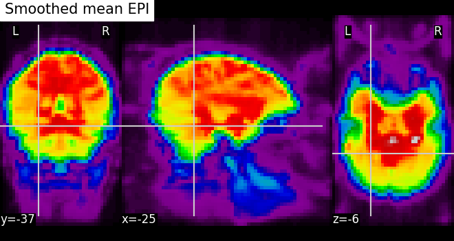
Functional MRI data can be considered “high dimensional” given the p-versus-n ratio (e.g., p=~20,000-200,000 voxels for n=1000 samples or less). In this setting, machine-learning algorithms can perform poorly due to the so-called curse of dimensionality. However, simple means from classical statistics can help reduce the number of voxels.

from nilearn.image import get_data

fmri_data = get_data(fmri_img)

# number of voxels being x*y*z, samples in 4th dimension
fmri_data.shape

(40, 64, 64, 1452)

Selecting features using a T-test

The Student’s t-test (scipy.stats.ttest_ind) is an established method to determine whether two distributions have a different mean value. It can be used to compare voxel time-series from two different experimental conditions (e.g., when houses or faces are shown to individuals during brain scanning). If the time-series distribution is similar in the two conditions, then the voxel is not very interesting to discriminate the condition.

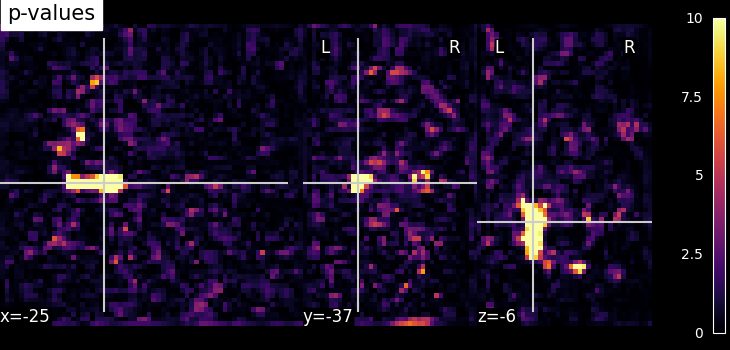
This test returns p-values that represent probabilities that the two time-series were not drawn from the same distribution. The lower the p-value, the more discriminative is the voxel in distinguishing the two conditions (faces and houses).

import numpy as np
from scipy import stats

_, p_values = stats.ttest_ind(
    fmri_data[..., haxby_labels == "face"],
    fmri_data[..., haxby_labels == "house"],
    axis=-1,
)

# Use a log scale for p-values
log_p_values = -np.log10(p_values)
# Set NAN values to zero
log_p_values[np.isnan(log_p_values)] = 0.0
log_p_values[log_p_values > 10.0] = 10.0

Visualize statistical p-values

Before visualizing, we transform the computed p-values to a Nifti-like image using function new_img_like from nilearn. First argument being a reference image and second argument should be p-values data to convert to a new image as output. This new image will have same header information as the reference image.

from nilearn.image import new_img_like

log_p_values_img = new_img_like(fmri_img, log_p_values)

Now, we visualize the log p-values image on the functional mean image as a background with coordinates given manually and a colorbar on the right side of the plot (by default, colorbar=True).

from nilearn.plotting import plot_stat_map

plot_stat_map(
    log_p_values_img,
    mean_img,
    title="p-values",
    cut_coords=cut_coords,
    cmap="inferno",
)

show()

Selecting features using f_classif

It is also possible to use the sklearn.feature_selection.f_classif function, which works for feature selection in multi-class settings.

Build a mask

Thresholding

We build the t-map to have better representation of voxels of interest, where voxels with lower p-values correspond to the most intense voxels. This can be done easily by applying a threshold to a t-map data in array.

Note that we use log p-values data; we force values below 5 to 0 by thresholding.

log_p_values[log_p_values < 5] = 0

Visualize the reduced voxels of interest using statistical image plotting function. As shown above, we first transform data in array to Nifti image.

log_p_values_img = new_img_like(fmri_img, log_p_values)

# Now, visualizing the created log p-values to image.
plot_stat_map(
    log_p_values_img,
    mean_img,
    title="Thresholded p-values",
    cut_coords=cut_coords,
    cmap="inferno",
)

show()

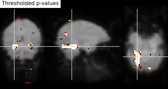
We can post-process the results obtained with simple operations such as mask intersection and dilation to regularize the mask definition. The idea of using these operations are to have more compact or sparser blobs.

Binarization and Intersection with Ventral Temporal (VT) mask

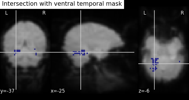
We now want to restrict our investigation to the VT area. The corresponding spatial mask is provided in haxby_dataset.mask_vt. We want to compute the intersection of this provided mask with our self-computed mask.

# self-computed mask
bin_p_values = log_p_values != 0
# VT mask
mask_vt_filename = haxby_dataset.mask_vt[0]

# The first step is to load VT mask and at the same time to convert the
# datatype from "number" to "boolean".
from nilearn.image import load_img

vt = get_data(load_img(mask_vt_filename)).astype(bool)

We can then use a logical “and” operation - numpy.logical_and - to keep only voxels that have been selected in both masks. In neuroimaging jargon, this is called an “AND conjunction”.

bin_p_values_and_vt = np.logical_and(bin_p_values, vt)

Visualizing the mask intersection results using plotting function plot_roi, a function which can be used for visualizing target specific voxels.

First, we create new image type of binarized and intersected mask (second argument) and use this created Nifti image type in visualization. Binarized values in data type boolean should be converted to int data type at the same time. Otherwise, an error will be raised.

bin_p_values_and_vt_img = new_img_like(
    fmri_img, bin_p_values_and_vt.astype(np.int32)
)
# We visualize the mask using the computed mean of functional images as
# background.
from nilearn.plotting import plot_roi

plot_roi(
    bin_p_values_and_vt_img,
    mean_img,
    cut_coords=cut_coords,
    title="Intersection with ventral temporal mask",
)

show()

Dilation

Thresholded functional brain images often contain scattered voxels across the brain. To consolidate such brain images towards more compact shapes, we use a morphological dilation. This is a common step to be sure not to forget voxels located on the edge of a ROI. In other words, such operations can fill “holes” in masked voxel representations.

# We use ndimage function from scipy Python library for mask dilation.
from scipy.ndimage import binary_dilation

# Input here is a binarized and intersected mask data
# from the previous section.
dil_bin_p_values_and_vt = binary_dilation(bin_p_values_and_vt)

# Now, we visualize the same using `plot_roi` with the data being converted
# to Nifti image. In all `new_img_like` calls, we use the same reference image.
dil_bin_p_values_and_vt_img = new_img_like(
    fmri_img, dil_bin_p_values_and_vt.astype(np.int32)
)
plot_roi(
    dil_bin_p_values_and_vt_img,
    mean_img,
    title="Dilated mask",
    cut_coords=cut_coords,
)

show()

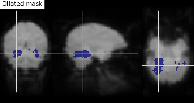
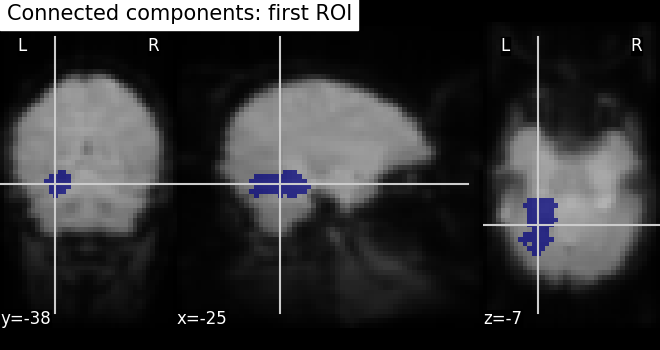
Finally, we end with splitting the connected ROIs to two hemispheres into two separate regions (ROIs). We use the function scipy.ndimage.label from the scipy Python library.

Identification of connected components

The function scipy.ndimage.label from the scipy Python library identifies immediately neighboring voxels in our voxels mask. It assigns a separate integer label to each one of them.

from scipy.ndimage import label

labels, _ = label(dil_bin_p_values_and_vt)

# we take first roi data with labels assigned as integer 1
first_roi_data = (labels == 5).astype(np.int32)

# Similarly, second roi data is assigned as integer 2
second_roi_data = (labels == 3).astype(np.int32)

Visualizing the connected components

First, we create a Nifti image type from first roi data in a array.

first_roi_img = new_img_like(fmri_img, first_roi_data)

Then, we visualize the same created Nifti image (first argument) with the mean of functional images as background (second argument). The cut_coords are the default now: coordinates are selected automatically and will be pointed exactly on the roi data.

plot_roi(first_roi_img, mean_img, title="Connected components: first ROI")

<nilearn.plotting.displays._slicers.OrthoSlicer object at 0x7febd3c16b90>

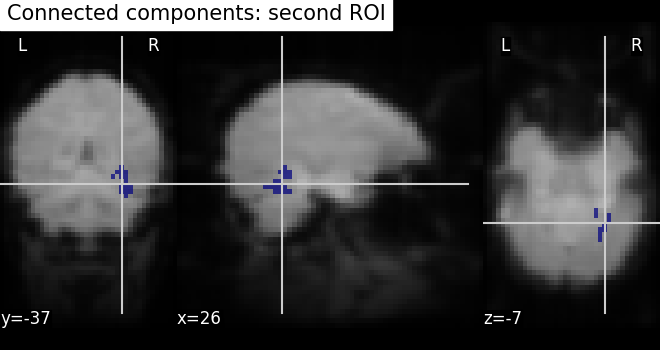
We do the same for the second roi data.

second_roi_img = new_img_like(fmri_img, second_roi_data)
plot_roi(second_roi_img, mean_img, title="Connected components: second ROI")

show()

Use the new ROIs to extract data maps in both ROIs

We extract data from ROIs using Nilearn’s NiftiLabelsMasker.

from nilearn.maskers import NiftiLabelsMasker

Before data extraction, we convert array labels to a Nifti like image. All inputs to NiftiLabelsMasker must be Nifti-like images or filenames to Nifti images. We use the same reference image as used above in previous sections.

labels_img = new_img_like(fmri_img, labels)

First, we initialize a masker with parameters suited for data extraction: labels as input image, resampling_target is None as the affine and shape/size are the same for all the data used here, time series signal processing parameters standardize and detrend are set to False.

masker = NiftiLabelsMasker(
    labels_img,
    resampling_target=None,
    standardize=None,
    detrend=False,
    verbose=1,
)

Preparing for data extraction: setting number of conditions, size, etc. from the Haxby dataset.

condition_names = haxby_labels.unique()
n_cond_img = fmri_data[..., haxby_labels == "house"].shape[-1]
n_conds = len(condition_names)

X1, X2 = np.zeros((n_cond_img, n_conds)), np.zeros((n_cond_img, n_conds))

Gathering data for each condition and then use fit_transform on each data. The transformer extracts data in condition maps where the target regions are specified by labels images.

for i, cond in enumerate(condition_names):
    cond_maps = new_img_like(
        fmri_img, fmri_data[..., haxby_labels == cond][..., :n_cond_img]
    )
    mask_data = masker.fit_transform(cond_maps)
    X1[:, i], X2[:, i] = mask_data[:, 0], mask_data[:, 1]
condition_names[np.where(condition_names == "scrambledpix")] = "scrambled"

\[NiftiLabelsMasker.wrapped] Loading regions from <nibabel.nifti1.Nifti1Image
object at 0x7febd988ebc0>
\[NiftiLabelsMasker.wrapped] Finished fit
\[NiftiLabelsMasker.wrapped] Loading data from <nibabel.nifti1.Nifti1Image
object at 0x7febe5e3c7c0>
\[NiftiLabelsMasker.wrapped] Extracting region signals
\[NiftiLabelsMasker.wrapped] Cleaning extracted signals
\[NiftiLabelsMasker.wrapped] Loading regions from <nibabel.nifti1.Nifti1Image
object at 0x7febd988ebc0>
\[NiftiLabelsMasker.wrapped] Finished fit
\[NiftiLabelsMasker.wrapped] Loading data from <nibabel.nifti1.Nifti1Image
object at 0x7febfe064130>
\[NiftiLabelsMasker.wrapped] Extracting region signals
\[NiftiLabelsMasker.wrapped] Cleaning extracted signals
\[NiftiLabelsMasker.wrapped] Loading regions from <nibabel.nifti1.Nifti1Image
object at 0x7febd988ebc0>
\[NiftiLabelsMasker.wrapped] Finished fit
\[NiftiLabelsMasker.wrapped] Loading data from <nibabel.nifti1.Nifti1Image
object at 0x7febe5e3e1a0>
\[NiftiLabelsMasker.wrapped] Extracting region signals
\[NiftiLabelsMasker.wrapped] Cleaning extracted signals
\[NiftiLabelsMasker.wrapped] Loading regions from <nibabel.nifti1.Nifti1Image
object at 0x7febd988ebc0>
\[NiftiLabelsMasker.wrapped] Finished fit
\[NiftiLabelsMasker.wrapped] Loading data from <nibabel.nifti1.Nifti1Image
object at 0x7febfe0665c0>
\[NiftiLabelsMasker.wrapped] Extracting region signals
\[NiftiLabelsMasker.wrapped] Cleaning extracted signals
\[NiftiLabelsMasker.wrapped] Loading regions from <nibabel.nifti1.Nifti1Image
object at 0x7febd988ebc0>
\[NiftiLabelsMasker.wrapped] Finished fit
\[NiftiLabelsMasker.wrapped] Loading data from <nibabel.nifti1.Nifti1Image
object at 0x7febb7121450>
\[NiftiLabelsMasker.wrapped] Extracting region signals
\[NiftiLabelsMasker.wrapped] Cleaning extracted signals
\[NiftiLabelsMasker.wrapped] Loading regions from <nibabel.nifti1.Nifti1Image
object at 0x7febd988ebc0>
\[NiftiLabelsMasker.wrapped] Finished fit
\[NiftiLabelsMasker.wrapped] Loading data from <nibabel.nifti1.Nifti1Image
object at 0x7febfe064100>
\[NiftiLabelsMasker.wrapped] Extracting region signals
\[NiftiLabelsMasker.wrapped] Cleaning extracted signals
\[NiftiLabelsMasker.wrapped] Loading regions from <nibabel.nifti1.Nifti1Image
object at 0x7febd988ebc0>
\[NiftiLabelsMasker.wrapped] Finished fit
\[NiftiLabelsMasker.wrapped] Loading data from <nibabel.nifti1.Nifti1Image
object at 0x7febfe064c40>
\[NiftiLabelsMasker.wrapped] Extracting region signals
\[NiftiLabelsMasker.wrapped] Cleaning extracted signals
\[NiftiLabelsMasker.wrapped] Loading regions from <nibabel.nifti1.Nifti1Image
object at 0x7febd988ebc0>
\[NiftiLabelsMasker.wrapped] Finished fit
\[NiftiLabelsMasker.wrapped] Loading data from <nibabel.nifti1.Nifti1Image
object at 0x7febffab2290>
\[NiftiLabelsMasker.wrapped] Extracting region signals
\[NiftiLabelsMasker.wrapped] Cleaning extracted signals
\[NiftiLabelsMasker.wrapped] Loading regions from <nibabel.nifti1.Nifti1Image
object at 0x7febd988ebc0>
\[NiftiLabelsMasker.wrapped] Finished fit
\[NiftiLabelsMasker.wrapped] Loading data from <nibabel.nifti1.Nifti1Image
object at 0x7febfe0651e0>
\[NiftiLabelsMasker.wrapped] Extracting region signals
\[NiftiLabelsMasker.wrapped] Cleaning extracted signals

Save the ROI ‘atlas’ to a Nifti file.

from pathlib import Path

output_dir = Path.cwd() / "results" / "plot_roi_extraction"
output_dir.mkdir(exist_ok=True, parents=True)
print(f"Output will be saved to: {output_dir}")

new_img_like(fmri_img, labels).to_filename(output_dir / "mask_atlas.nii.gz")

Output will be saved to: /home/runner/work/nilearn/nilearn/examples/06_manipulating_images/results/plot_roi_extraction

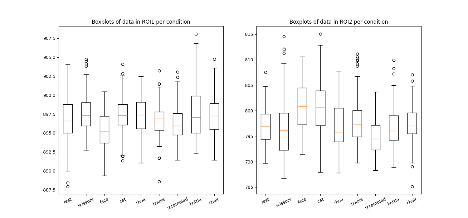
Plot the average in the different condition names.

import matplotlib.pyplot as plt

plt.figure(figsize=(15, 7))
for i in np.arange(2):
    plt.subplot(1, 2, i + 1)
    plt.boxplot(X1 if i == 0 else X2)
    plt.xticks(
        np.arange(len(condition_names)) + 1, condition_names, rotation=25
    )
    plt.title(f"Boxplots of data in ROI{int(i + 1)} per condition")

show()

Estimated memory usage: 2398 MB