Note
Go to the end to download the full example code. or to run this example in your browser via Binder
Default Mode Network extraction of ADHD dataset
This example shows a full step-by-step workflow of fitting a GLM to signal extracted from a seed on the Posterior Cingulate Cortex and saving the results. More precisely, this example shows how to use a signal extracted from a seed region as the regressor in a GLM to determine the correlation of each region in the dataset with the seed region.
More specifically:
A sequence of fMRI volumes are loaded.
A design matrix with the Posterior Cingulate Cortex seed is defined.
A GLM is applied to the dataset (effect/covariance, then contrast estimation).
The Default Mode Network is displayed.
import numpy as np

from nilearn import plotting
from nilearn.datasets import fetch_adhd
from nilearn.glm.first_level import (
    FirstLevelModel,
    make_first_level_design_matrix,
)
from nilearn.maskers import NiftiSpheresMasker
Prepare data and analysis parameters
Prepare the data.
For more information see the dataset description.
adhd_dataset = fetch_adhd(n_subjects=1)

# Prepare seed
pcc_coords = (0, -53, 26)
[fetch_adhd] Dataset directory found:
/home/runner/work/nilearn/nilearn/nilearn_data/adhd
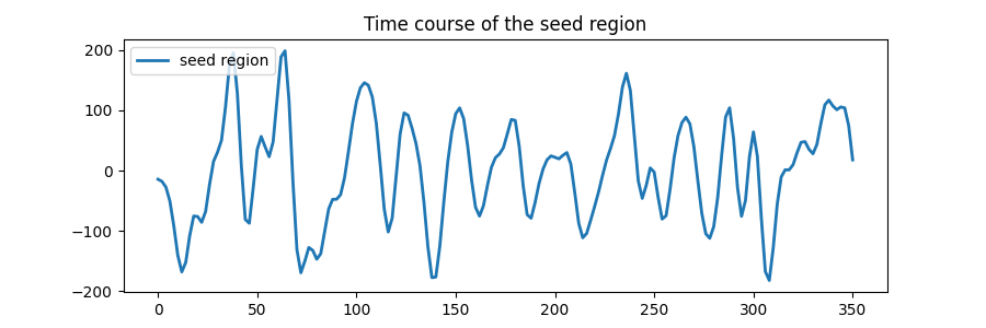
Extract the seed region’s time course
Extract the time course of the seed region.
seed_masker = NiftiSpheresMasker(
    [pcc_coords],
    radius=10,
    detrend=True,
    low_pass=0.1,
    high_pass=0.01,
    t_r=adhd_dataset.t_r,
    memory="nilearn_cache",
    memory_level=1,
    verbose=1,
)
seed_time_series = seed_masker.fit_transform(adhd_dataset.func[0])

n_scans = seed_time_series.shape[0]
frametimes = np.linspace(0, (n_scans - 1) * adhd_dataset.t_r, n_scans)
\[NiftiSpheresMasker.wrapped] Finished fit
/home/runner/work/nilearn/nilearn/examples/04_glm_first_level/plot_adhd_dmn.py:61: FutureWarning:

boolean values for 'standardize' will be deprecated in nilearn 0.15.0.
Use 'zscore_sample' instead of 'True' or use 'None' instead of 'False'.

________________________________________________________________________________
[Memory] Calling nilearn.maskers.base_masker.filter_and_extract...
filter_and_extract('/home/runner/work/nilearn/nilearn/nilearn_data/adhd/data/0010042/0010042_rest_tshift_RPI_voreg_mni.nii.gz',
<nilearn.maskers.nifti_spheres_masker._ExtractionFunctor object at 0x7f2b0389d9f0>,
{ 'allow_overlap': False,
  'clean_args': None,
  'clean_kwargs': {},
  'detrend': True,
  'dtype': None,
  'high_pass': 0.01,
  'high_variance_confounds': False,
  'low_pass': 0.1,
  'mask_img': None,
  'radius': 10,
  'reports': True,
  'seeds': [(0, -53, 26)],
  'smoothing_fwhm': None,
  'standardize': False,
  'standardize_confounds': True,
  't_r': 2.0}, confounds=None, sample_mask=None, dtype=None, sklearn_output_config=None, memory=Memory(location=nilearn_cache/joblib), memory_level=1, verbose=1)
\[NiftiSpheresMasker.wrapped] Loading data from '/home/runner/work/nilearn/nilea
rn/nilearn_data/adhd/data/0010042/0010042_rest_tshift_RPI_voreg_mni.nii.gz'
\[NiftiSpheresMasker.wrapped] Extracting region signals
\[NiftiSpheresMasker.wrapped] Cleaning extracted signals
/home/runner/work/nilearn/nilearn/examples/04_glm_first_level/plot_adhd_dmn.py:61: FutureWarning:

boolean values for 'standardize' will be deprecated in nilearn 0.15.0.
Use 'zscore_sample' instead of 'True' or use 'None' instead of 'False'.

_______________________________________________filter_and_extract - 3.9s, 0.1min
Plot the time course of the seed region.
import matplotlib.pyplot as plt

fig = plt.figure(figsize=(9, 3))
ax = fig.add_subplot(111)
ax.plot(frametimes, seed_time_series, linewidth=2, label="seed region")
ax.legend(loc=2)
ax.set_title("Time course of the seed region")
plt.show()
Estimate contrasts
Specify the contrasts.
design_matrix = make_first_level_design_matrix(
    frametimes,
    hrf_model="spm",
    add_regs=seed_time_series,
    add_reg_names=["pcc_seed"],
)
dmn_contrast = np.array([1] + [0] * (design_matrix.shape[1] - 1))
contrasts = {"seed_based_glm": dmn_contrast}
Perform first level analysis
Setup and fit GLM.
first_level_model = FirstLevelModel(verbose=1)
first_level_model = first_level_model.fit(
    run_imgs=adhd_dataset.func[0], design_matrices=design_matrix
)
\[FirstLevelModel.fit] Computing run 1 out of 1 runs (go take a coffee, a big
one).
\[FirstLevelModel.fit] Performing mask computation.
\[FirstLevelModel.fit] Masking took 0 seconds.
/home/runner/work/nilearn/nilearn/examples/04_glm_first_level/plot_adhd_dmn.py:95: UserWarning:

Mean values of 0 observed. The data have probably been centered. Scaling might not work as expected.

\[FirstLevelModel.fit] Performing GLM computation.
\[FirstLevelModel.fit] GLM took 1 seconds.
\[FirstLevelModel.fit] Computation of 1 runs done in 00 HR 00 MIN 03 SEC.
Estimate the contrast.
print("Contrast seed_based_glm computed.")
z_map = first_level_model.compute_contrast(
    contrasts["seed_based_glm"], output_type="z_score"
)
Contrast seed_based_glm computed.
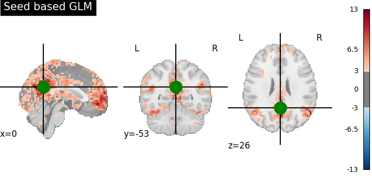
Saving snapshots of the contrasts
from pathlib import Path

display = plotting.plot_stat_map(
    z_map, threshold=3.0, title="Seed based GLM", cut_coords=pcc_coords
)
display.add_markers(
    marker_coords=[pcc_coords], marker_color="g", marker_size=300
)

output_dir = Path.cwd() / "results" / "plot_adhd_dmn"
output_dir.mkdir(exist_ok=True, parents=True)
filename = "dmn_z_map.png"
display.savefig(output_dir / filename)
print(f"Save z-map in '{filename}'.")
Save z-map in 'dmn_z_map.png'.
Generating a report
It can be useful to quickly generate a portable, ready-to-view report with most of the pertinent information. This is easy to do if you have a fitted model and the list of contrasts, which we do here.
report = first_level_model.generate_report(
    contrasts=contrasts,
    title="ADHD DMN Report",
    cluster_threshold=15,
    min_distance=8.0,
    plot_type="glass",
)
Note
The generated report can be:
displayed in a Notebook,
opened in a browser using the
.open_in_browser()method,or saved to a file using the
.save_as_html(output_filepath)method.
ADHD DMN Report Implement the General Linear Model for single run :term:`fMRI` data.
Description
Data were analyzed using Nilearn (version= 0.14.1; RRID:SCR_001362).
At the subject level, a mass univariate analysis was performed with a linear regression at each voxel of the brain, using generalized least squares with a global ar1 noise model to account for temporal auto-correlation and a cosine drift model (high pass filter=0.01 Hz).
Model details
| Value | |
|---|---|
| Parameter | |
| drift_model | cosine |
| high_pass (Hertz) | 0.01 |
| hrf_model | glover |
| noise_model | ar1 |
| signal_scaling | 0 |
| slice_time_ref | 0.0 |
| standardize | False |
Design Matrix

correlation matrix

Contrasts
.")
Mask

The mask includes 62546 voxels (23.0 %) of the image.
Statistical Maps
seed_based_glm

Cluster Table
| Height control | fpr |
|---|---|
| α | 0.001 |
| Threshold (computed) | 3.09 |
| Cluster size threshold (voxels) | 15 |
| Minimum distance (mm) | 8.0 |
| Cluster ID | X | Y | Z | Peak Stat | Cluster Size (mm3) |
|---|---|---|---|---|---|
| 1 | 3.0 | -54.0 | 18.0 | 13.01 | 113616 |
| 1a | 0.0 | -57.0 | 30.0 | 12.68 | |
| 1b | 0.0 | -48.0 | 30.0 | 11.96 | |
| 1c | -3.0 | -51.0 | 18.0 | 11.91 | |
| 2 | 0.0 | 51.0 | -6.0 | 11.08 | 32103 |
| 2a | 3.0 | 69.0 | 3.0 | 10.62 | |
| 2b | 0.0 | 57.0 | 3.0 | 10.31 | |
| 2c | 0.0 | 63.0 | 15.0 | 10.12 | |
| 3 | 57.0 | -66.0 | 27.0 | 10.91 | 7209 |
| 3a | 48.0 | -57.0 | 30.0 | 8.99 | |
| 3b | 51.0 | -69.0 | 27.0 | 8.51 | |
| 3c | 45.0 | -69.0 | 39.0 | 6.39 | |
| 4 | 48.0 | -66.0 | -21.0 | 10.71 | 4563 |
| 4a | 42.0 | -54.0 | -24.0 | 7.29 | |
| 4b | 51.0 | -60.0 | -21.0 | 6.42 | |
| 4c | 33.0 | -78.0 | -36.0 | 5.37 | |
| 5 | -42.0 | 24.0 | -24.0 | 10.71 | 4077 |
| 5a | -57.0 | 3.0 | -15.0 | 7.02 | |
| 5b | -42.0 | 9.0 | -30.0 | 5.87 | |
| 5c | -45.0 | 3.0 | -45.0 | 5.67 | |
| 6 | 42.0 | 27.0 | -24.0 | 10.71 | 972 |
| 6a | 39.0 | 36.0 | -15.0 | 7.45 | |
| 6b | 39.0 | 21.0 | -18.0 | 4.72 | |
| 7 | -12.0 | 39.0 | 54.0 | 8.52 | 4590 |
| 7a | -24.0 | 30.0 | 48.0 | 8.51 | |
| 7b | -18.0 | 30.0 | 42.0 | 8.39 | |
| 7c | -15.0 | 30.0 | 51.0 | 7.87 | |
| 8 | 60.0 | -3.0 | -12.0 | 7.94 | 3186 |
| 8a | 66.0 | -18.0 | -6.0 | 6.62 | |
| 8b | 66.0 | -27.0 | -3.0 | 6.35 | |
| 8c | 57.0 | -12.0 | -9.0 | 6.15 | |
| 9 | 51.0 | 9.0 | -39.0 | 6.73 | 1053 |
| 9a | 51.0 | 9.0 | -27.0 | 3.30 | |
| 10 | -24.0 | -75.0 | 51.0 | 6.65 | 594 |
| 10a | -15.0 | -75.0 | 57.0 | 4.84 | |
| 10b | -36.0 | -72.0 | 51.0 | 4.52 | |
| 11 | 21.0 | -33.0 | 0.0 | 6.54 | 2295 |
| 11a | 21.0 | -21.0 | -12.0 | 5.72 | |
| 11b | 30.0 | -27.0 | -9.0 | 5.15 | |
| 11c | 9.0 | -30.0 | -6.0 | 4.64 | |
| 12 | -39.0 | 9.0 | 39.0 | 6.36 | 1809 |
| 12a | -48.0 | 9.0 | 42.0 | 5.19 | |
| 12b | -36.0 | 24.0 | 18.0 | 4.75 | |
| 13 | -39.0 | -36.0 | -21.0 | 6.27 | 1215 |
| 13a | -42.0 | -24.0 | -21.0 | 5.48 | |
| 13b | -39.0 | -12.0 | -36.0 | 4.78 | |
| 14 | 36.0 | 9.0 | 36.0 | 6.25 | 1026 |
| 14a | 36.0 | 18.0 | 36.0 | 5.15 | |
| 14b | 39.0 | 9.0 | 42.0 | 5.04 | |
| 14c | 48.0 | 12.0 | 45.0 | 4.66 | |
| 15 | -9.0 | -51.0 | -39.0 | 6.10 | 1404 |
| 15a | 3.0 | -60.0 | -51.0 | 4.72 | |
| 16 | -51.0 | -78.0 | 18.0 | 6.06 | 891 |
| 16a | -54.0 | -66.0 | 6.0 | 4.13 | |
| 16b | -48.0 | -63.0 | 0.0 | 4.07 | |
| 16c | -51.0 | -75.0 | 9.0 | 3.89 | |
| 17 | 51.0 | -45.0 | 36.0 | 5.98 | 675 |
| 17a | 57.0 | -45.0 | 27.0 | 4.64 | |
| 18 | -15.0 | 57.0 | 30.0 | 5.94 | 1458 |
| 18a | -21.0 | 54.0 | 36.0 | 5.72 | |
| 18b | -9.0 | 51.0 | 33.0 | 4.79 | |
| 18c | -27.0 | 54.0 | 30.0 | 4.70 | |
| 19 | 33.0 | -36.0 | -12.0 | 5.78 | 594 |
| 19a | 33.0 | -30.0 | -18.0 | 4.83 | |
| 20 | -27.0 | 54.0 | 0.0 | 5.36 | 837 |
| 20a | -24.0 | 54.0 | 9.0 | 3.98 | |
| 21 | 27.0 | -69.0 | -6.0 | 5.32 | 2241 |
| 21a | 21.0 | -75.0 | -9.0 | 5.22 | |
| 21b | 27.0 | -57.0 | -12.0 | 4.83 | |
| 21c | 33.0 | -51.0 | -9.0 | 4.52 | |
| 22 | 48.0 | -66.0 | -9.0 | 5.00 | 594 |
| 22a | 48.0 | -75.0 | -12.0 | 4.50 | |
| 22b | 48.0 | -60.0 | -12.0 | 4.36 | |
| 23 | -3.0 | -9.0 | 72.0 | 4.76 | 648 |
| 23a | 0.0 | 3.0 | 69.0 | 3.87 | |
| 23b | -3.0 | -9.0 | 63.0 | 3.59 | |
| 24 | -42.0 | -60.0 | -6.0 | 4.76 | 567 |
| 25 | -9.0 | -102.0 | -3.0 | 4.52 | 486 |
| 25a | -6.0 | -102.0 | 6.0 | 3.76 |
About
- Date preprocessed:
Total running time of the script: (0 minutes 15.280 seconds)
Estimated memory usage: 509 MB