Note
Go to the end to download the full example code. or to run this example in your browser via Binder
Example of generic design in second-level models
This example shows the results obtained in a group analysis using a more complex contrast than a one- or two-sample t test. We use the [left button press (auditory cue)] task from the Localizer dataset and seek association between the contrast values and a variate that measures the speed of pseudo-word reading. No confounding variate is included in the model.
At first, we need to load the Localizer contrasts.
from nilearn.datasets import fetch_localizer_contrasts

n_samples = 94
localizer_dataset = fetch_localizer_contrasts(
    ["left button press (auditory cue)"],
    n_subjects=n_samples,
)
[fetch_localizer_contrasts] Dataset found in
/home/runner/nilearn_data/brainomics_localizer
[fetch_localizer_contrasts] Downloading data from
https://osf.io/download/5d27da3a114a4200190453ab/ ...
[fetch_localizer_contrasts]  ...done. (3 seconds, 0 min)

[fetch_localizer_contrasts] Downloading data from
https://osf.io/download/5d27ebc3114a42001704a18d/ ...
[fetch_localizer_contrasts]  ...done. (2 seconds, 0 min)

[fetch_localizer_contrasts] Downloading data from
https://osf.io/download/5d27f1f0114a42001804603e/ ...
[fetch_localizer_contrasts]  ...done. (2 seconds, 0 min)

[fetch_localizer_contrasts] Downloading data from
https://osf.io/download/5d28092e45253a001c3e597f/ ...
[fetch_localizer_contrasts]  ...done. (2 seconds, 0 min)

[fetch_localizer_contrasts] Downloading data from
https://osf.io/download/5d281a531c5b4a001c9ea662/ ...
[fetch_localizer_contrasts]  ...done. (3 seconds, 0 min)

[fetch_localizer_contrasts] Downloading data from
https://osf.io/download/5d28295aa26b340018087ef4/ ...
[fetch_localizer_contrasts]  ...done. (2 seconds, 0 min)

[fetch_localizer_contrasts] Downloading data from
https://osf.io/download/5d283473a26b34001609ed88/ ...
[fetch_localizer_contrasts]  ...done. (3 seconds, 0 min)

[fetch_localizer_contrasts] Downloading data from
https://osf.io/download/5d284374114a42001605f4d2/ ...
[fetch_localizer_contrasts]  ...done. (2 seconds, 0 min)

[fetch_localizer_contrasts] Downloading data from
https://osf.io/download/5d28590d114a4200160607da/ ...
[fetch_localizer_contrasts]  ...done. (2 seconds, 0 min)

[fetch_localizer_contrasts] Downloading data from
https://osf.io/download/5d285a53114a4200160608be/ ...
[fetch_localizer_contrasts]  ...done. (2 seconds, 0 min)

[fetch_localizer_contrasts] Downloading data from
https://osf.io/download/5d286f35a26b34001908e5c1/ ...
[fetch_localizer_contrasts]  ...done. (2 seconds, 0 min)

[fetch_localizer_contrasts] Downloading data from
https://osf.io/download/5d2888ce1c5b4a001b9f789c/ ...
[fetch_localizer_contrasts]  ...done. (2 seconds, 0 min)

[fetch_localizer_contrasts] Downloading data from
https://osf.io/download/5d289b2945253a00193d32ac/ ...
[fetch_localizer_contrasts]  ...done. (3 seconds, 0 min)

[fetch_localizer_contrasts] Downloading data from
https://osf.io/download/5d28a00245253a001c3efac9/ ...
[fetch_localizer_contrasts]  ...done. (2 seconds, 0 min)

[fetch_localizer_contrasts] Downloading data from
https://osf.io/download/5d28bc0145253a00193d53ab/ ...
[fetch_localizer_contrasts]  ...done. (2 seconds, 0 min)

[fetch_localizer_contrasts] Downloading data from
https://osf.io/download/5d28cfd91c5b4a001c9f404d/ ...
[fetch_localizer_contrasts]  ...done. (2 seconds, 0 min)

[fetch_localizer_contrasts] Downloading data from
https://osf.io/download/5d28db3ba26b34001808f444/ ...
[fetch_localizer_contrasts]  ...done. (3 seconds, 0 min)

[fetch_localizer_contrasts] Downloading data from
https://osf.io/download/5d28f0bc1c5b4a001b9fd7f3/ ...
[fetch_localizer_contrasts]  ...done. (2 seconds, 0 min)

[fetch_localizer_contrasts] Downloading data from
https://osf.io/download/5d28ffc245253a00193d7dac/ ...
[fetch_localizer_contrasts]  ...done. (3 seconds, 0 min)

[fetch_localizer_contrasts] Downloading data from
https://osf.io/download/5d2909cd1c5b4a001b9fe6c5/ ...
[fetch_localizer_contrasts]  ...done. (2 seconds, 0 min)

[fetch_localizer_contrasts] Downloading data from
https://osf.io/download/5d2919e2114a42001606b46c/ ...
[fetch_localizer_contrasts]  ...done. (2 seconds, 0 min)

[fetch_localizer_contrasts] Downloading data from
https://osf.io/download/5d2928bc45253a001b3cf010/ ...
[fetch_localizer_contrasts]  ...done. (2 seconds, 0 min)

[fetch_localizer_contrasts] Downloading data from
https://osf.io/download/5d293a50a26b34001909682a/ ...
[fetch_localizer_contrasts]  ...done. (2 seconds, 0 min)

[fetch_localizer_contrasts] Downloading data from
https://osf.io/download/5d29492fa26b34001709070f/ ...
[fetch_localizer_contrasts]  ...done. (2 seconds, 0 min)

[fetch_localizer_contrasts] Downloading data from
https://osf.io/download/5d295328114a42001606dd9a/ ...
[fetch_localizer_contrasts]  ...done. (3 seconds, 0 min)

[fetch_localizer_contrasts] Downloading data from
https://osf.io/download/5d2c37031c5b4a001ca0da2b/ ...
[fetch_localizer_contrasts]  ...done. (3 seconds, 0 min)

[fetch_localizer_contrasts] Downloading data from
https://osf.io/download/5d2c442e114a420017071134/ ...
[fetch_localizer_contrasts]  ...done. (2 seconds, 0 min)

[fetch_localizer_contrasts] Downloading data from
https://osf.io/download/5d2c5c431c5b4a001da257a5/ ...
[fetch_localizer_contrasts]  ...done. (3 seconds, 0 min)

[fetch_localizer_contrasts] Downloading data from
https://osf.io/download/5d2c6c2645253a001c42460f/ ...
[fetch_localizer_contrasts]  ...done. (2 seconds, 0 min)

[fetch_localizer_contrasts] Downloading data from
https://osf.io/download/5d2ec286251f0e001604a189/ ...
[fetch_localizer_contrasts]  ...done. (3 seconds, 0 min)

[fetch_localizer_contrasts] Downloading data from
https://osf.io/download/5d2ed2875d2cdc001702b4c5/ ...
[fetch_localizer_contrasts]  ...done. (2 seconds, 0 min)

[fetch_localizer_contrasts] Downloading data from
https://osf.io/download/5d341711a667db0017fc816f/ ...
[fetch_localizer_contrasts]  ...done. (2 seconds, 0 min)

[fetch_localizer_contrasts] Downloading data from
https://osf.io/download/5d34294d835aff001958add9/ ...
[fetch_localizer_contrasts]  ...done. (2 seconds, 0 min)

[fetch_localizer_contrasts] Downloading data from
https://osf.io/download/5d2ef8925d2cdc001702e0a5/ ...
[fetch_localizer_contrasts]  ...done. (3 seconds, 0 min)

[fetch_localizer_contrasts] Downloading data from
https://osf.io/download/5d2f0851251f0e0018044fe4/ ...
[fetch_localizer_contrasts]  ...done. (2 seconds, 0 min)

[fetch_localizer_contrasts] Downloading data from
https://osf.io/download/5d2f26e4a667db0017f72ae9/ ...
[fetch_localizer_contrasts]  ...done. (2 seconds, 0 min)

[fetch_localizer_contrasts] Downloading data from
https://osf.io/download/5d2f358c251f0e001704a76a/ ...
[fetch_localizer_contrasts]  ...done. (2 seconds, 0 min)

[fetch_localizer_contrasts] Downloading data from
https://osf.io/download/5d2f41d2835aff001a52da0c/ ...
[fetch_localizer_contrasts]  ...done. (2 seconds, 0 min)

[fetch_localizer_contrasts] Downloading data from
https://osf.io/download/5d2f5acc835aff0018532004/ ...
[fetch_localizer_contrasts]  ...done. (2 seconds, 0 min)

[fetch_localizer_contrasts] Downloading data from
https://osf.io/download/5d2f692d835aff00175372e9/ ...
[fetch_localizer_contrasts]  ...done. (2 seconds, 0 min)

[fetch_localizer_contrasts] Downloading data from
https://osf.io/download/5d2f7456835aff0017537992/ ...
[fetch_localizer_contrasts]  ...done. (2 seconds, 0 min)

[fetch_localizer_contrasts] Downloading data from
https://osf.io/download/5d2f8881a667db0018f6b634/ ...
[fetch_localizer_contrasts]  ...done. (2 seconds, 0 min)

[fetch_localizer_contrasts] Downloading data from
https://osf.io/download/5d2f9552251f0e001605bb64/ ...
[fetch_localizer_contrasts]  ...done. (3 seconds, 0 min)

[fetch_localizer_contrasts] Downloading data from
https://osf.io/download/5d2faf785d2cdc0017039bb1/ ...
[fetch_localizer_contrasts]  ...done. (2 seconds, 0 min)

[fetch_localizer_contrasts] Downloading data from
https://osf.io/download/5d2fbffd835aff0018535ef5/ ...
[fetch_localizer_contrasts]  ...done. (3 seconds, 0 min)

[fetch_localizer_contrasts] Downloading data from
https://osf.io/download/5d2fc225a667db001af6222a/ ...
[fetch_localizer_contrasts]  ...done. (2 seconds, 0 min)

[fetch_localizer_contrasts] Downloading data from
https://osf.io/download/5d2fdd77835aff00195494d4/ ...
[fetch_localizer_contrasts]  ...done. (2 seconds, 0 min)

[fetch_localizer_contrasts] Downloading data from
https://osf.io/download/5d2fe5d5a667db0017f80f32/ ...
[fetch_localizer_contrasts]  ...done. (2 seconds, 0 min)

[fetch_localizer_contrasts] Downloading data from
https://osf.io/download/5d2ff3ea835aff0018538140/ ...
[fetch_localizer_contrasts]  ...done. (2 seconds, 0 min)

[fetch_localizer_contrasts] Downloading data from
https://osf.io/download/5d301049a667db0019f67ca0/ ...
[fetch_localizer_contrasts]  ...done. (2 seconds, 0 min)

[fetch_localizer_contrasts] Downloading data from
https://osf.io/download/5d3021b65d2cdc00190344d6/ ...
[fetch_localizer_contrasts]  ...done. (2 seconds, 0 min)

[fetch_localizer_contrasts] Downloading data from
https://osf.io/download/5d302afe5d2cdc0018030034/ ...
[fetch_localizer_contrasts]  ...done. (2 seconds, 0 min)

[fetch_localizer_contrasts] Downloading data from
https://osf.io/download/5d303ad4835aff001853bca4/ ...
[fetch_localizer_contrasts]  ...done. (2 seconds, 0 min)

[fetch_localizer_contrasts] Downloading data from
https://osf.io/download/5d304f845d2cdc001a032801/ ...
[fetch_localizer_contrasts]  ...done. (2 seconds, 0 min)

[fetch_localizer_contrasts] Downloading data from
https://osf.io/download/5d3058cd835aff001853d4c7/ ...
[fetch_localizer_contrasts]  ...done. (3 seconds, 0 min)

[fetch_localizer_contrasts] Downloading data from
https://osf.io/download/5d306f15a667db0018f78b4d/ ...
[fetch_localizer_contrasts]  ...done. (3 seconds, 0 min)

[fetch_localizer_contrasts] Downloading data from
https://osf.io/download/5d307f8b251f0e00190519ca/ ...
[fetch_localizer_contrasts]  ...done. (2 seconds, 0 min)

[fetch_localizer_contrasts] Downloading data from
https://osf.io/download/5d309cb5251f0e001606fe4b/ ...
[fetch_localizer_contrasts]  ...done. (2 seconds, 0 min)

[fetch_localizer_contrasts] Downloading data from
https://osf.io/download/5d30a667251f0e00190534dc/ ...
[fetch_localizer_contrasts]  ...done. (2 seconds, 0 min)

[fetch_localizer_contrasts] Downloading data from
https://osf.io/download/5d30bb07251f0e001705df42/ ...
[fetch_localizer_contrasts]  ...done. (2 seconds, 0 min)

[fetch_localizer_contrasts] Downloading data from
https://osf.io/download/5d30df37251f0e001705fd72/ ...
[fetch_localizer_contrasts]  ...done. (2 seconds, 0 min)

[fetch_localizer_contrasts] Downloading data from
https://osf.io/download/5d30e232a667db0018f7f2a9/ ...
[fetch_localizer_contrasts]  ...done. (3 seconds, 0 min)

[fetch_localizer_contrasts] Downloading data from
https://osf.io/download/5d30f7ec251f0e001805e3cd/ ...
[fetch_localizer_contrasts]  ...done. (2 seconds, 0 min)

[fetch_localizer_contrasts] Downloading data from
https://osf.io/download/5d3116dca667db0018f81c29/ ...
[fetch_localizer_contrasts]  ...done. (2 seconds, 0 min)

[fetch_localizer_contrasts] Downloading data from
https://osf.io/download/5d312688251f0e0016079f29/ ...
[fetch_localizer_contrasts]  ...done. (2 seconds, 0 min)

[fetch_localizer_contrasts] Downloading data from
https://osf.io/download/5d3134fe5d2cdc001705393d/ ...
[fetch_localizer_contrasts]  ...done. (2 seconds, 0 min)

[fetch_localizer_contrasts] Downloading data from
https://osf.io/download/5d3143f9835aff00195630ce/ ...
[fetch_localizer_contrasts]  ...done. (2 seconds, 0 min)

[fetch_localizer_contrasts] Downloading data from
https://osf.io/download/5d315ac0835aff001754e139/ ...
[fetch_localizer_contrasts]  ...done. (2 seconds, 0 min)

[fetch_localizer_contrasts] Downloading data from
https://osf.io/download/5d3160bc835aff00195649cf/ ...
[fetch_localizer_contrasts]  ...done. (2 seconds, 0 min)

[fetch_localizer_contrasts] Downloading data from
https://osf.io/download/5d317bb2251f0e001608002e/ ...
[fetch_localizer_contrasts]  ...done. (2 seconds, 0 min)

[fetch_localizer_contrasts] Downloading data from
https://osf.io/download/5d318a6c251f0e001905b6ed/ ...
[fetch_localizer_contrasts]  ...done. (2 seconds, 0 min)

[fetch_localizer_contrasts] Downloading data from
https://osf.io/download/5d31962da667db0017fa303d/ ...
[fetch_localizer_contrasts]  ...done. (2 seconds, 0 min)

[fetch_localizer_contrasts] Downloading data from
https://osf.io/download/5d31abe45d2cdc0019046202/ ...
[fetch_localizer_contrasts]  ...done. (2 seconds, 0 min)

[fetch_localizer_contrasts] Downloading data from
https://osf.io/download/5d31cdeea667db001af75ab9/ ...
[fetch_localizer_contrasts]  ...done. (2 seconds, 0 min)

[fetch_localizer_contrasts] Downloading data from
https://osf.io/download/5d31dc83835aff001956e6c5/ ...
[fetch_localizer_contrasts]  ...done. (2 seconds, 0 min)

[fetch_localizer_contrasts] Downloading data from
https://osf.io/download/5d31fefea667db0018f8ea9f/ ...
[fetch_localizer_contrasts]  ...done. (2 seconds, 0 min)

[fetch_localizer_contrasts] Downloading data from
https://osf.io/download/5d32072b5d2cdc0018043969/ ...
[fetch_localizer_contrasts]  ...done. (3 seconds, 0 min)

[fetch_localizer_contrasts] Downloading data from
https://osf.io/download/5d3219b4a667db0018f8ff1f/ ...
[fetch_localizer_contrasts]  ...done. (2 seconds, 0 min)

[fetch_localizer_contrasts] Downloading data from
https://osf.io/download/5d3234f3835aff00175590f0/ ...
[fetch_localizer_contrasts]  ...done. (2 seconds, 0 min)

[fetch_localizer_contrasts] Downloading data from
https://osf.io/download/5d323d06251f0e001706f0be/ ...
[fetch_localizer_contrasts]  ...done. (2 seconds, 0 min)

[fetch_localizer_contrasts] Downloading data from
https://osf.io/download/5d324e77251f0e001806e5e7/ ...
[fetch_localizer_contrasts]  ...done. (2 seconds, 0 min)

[fetch_localizer_contrasts] Downloading data from
https://osf.io/download/5d326b70835aff00195762f8/ ...
[fetch_localizer_contrasts]  ...done. (2 seconds, 0 min)

[fetch_localizer_contrasts] Downloading data from
https://osf.io/download/5d32731a5d2cdc001a0472bb/ ...
[fetch_localizer_contrasts]  ...done. (2 seconds, 0 min)

[fetch_localizer_contrasts] Downloading data from
https://osf.io/download/5d3286b7251f0e001906427f/ ...
[fetch_localizer_contrasts]  ...done. (2 seconds, 0 min)

[fetch_localizer_contrasts] Downloading data from
https://osf.io/download/5d3298815d2cdc001804700c/ ...
[fetch_localizer_contrasts]  ...done. (3 seconds, 0 min)

[fetch_localizer_contrasts] Downloading data from
https://osf.io/download/5d32ab6ea667db0017fb59e8/ ...
[fetch_localizer_contrasts]  ...done. (2 seconds, 0 min)

[fetch_localizer_contrasts] Downloading data from
https://osf.io/download/5d32bb275d2cdc001a049841/ ...
[fetch_localizer_contrasts]  ...done. (3 seconds, 0 min)

[fetch_localizer_contrasts] Downloading data from
https://osf.io/download/5d32d901a667db0018f9684f/ ...
[fetch_localizer_contrasts]  ...done. (2 seconds, 0 min)

[fetch_localizer_contrasts] Downloading data from
https://osf.io/download/5d32e9d3835aff001957cd79/ ...
[fetch_localizer_contrasts]  ...done. (2 seconds, 0 min)

[fetch_localizer_contrasts] Downloading data from
https://osf.io/download/5d32f34f835aff001755ee97/ ...
[fetch_localizer_contrasts]  ...done. (2 seconds, 0 min)

[fetch_localizer_contrasts] Downloading data from
https://osf.io/download/5d3306db5d2cdc001706c36f/ ...
[fetch_localizer_contrasts]  ...done. (2 seconds, 0 min)

[fetch_localizer_contrasts] Downloading data from
https://osf.io/download/5d332373251f0e001609acbd/ ...
[fetch_localizer_contrasts]  ...done. (2 seconds, 0 min)

[fetch_localizer_contrasts] Downloading data from
https://osf.io/download/5d332b7e835aff001957feec/ ...
[fetch_localizer_contrasts]  ...done. (2 seconds, 0 min)
Let’s print basic information on the dataset.
print(
    "First contrast nifti image (3D) is located "
    f"at: {localizer_dataset.cmaps[0]}"
)
First contrast nifti image (3D) is located at: /home/runner/nilearn_data/brainomics_localizer/brainomics_data/S01/cmaps_LeftAuditoryClick.nii.gz
we also need to load the behavioral variable.
tested_var = localizer_dataset.ext_vars["pseudo"]
print(tested_var)
0     15.0
1     16.0
2     14.0
3     19.0
4     16.0
      ...
89    12.0
90    16.0
91    13.0
92    25.0
93    21.0
Name: pseudo, Length: 94, dtype: float64
It is worth to do a quality check and remove subjects with missing values.
import numpy as np

mask_quality_check = np.where(np.logical_not(np.isnan(tested_var)))[0]
n_samples = mask_quality_check.size
contrast_map_filenames = [
    localizer_dataset.cmaps[i] for i in mask_quality_check
]
tested_var = tested_var[mask_quality_check].to_numpy().reshape((-1, 1))
print(f"Actual number of subjects after quality check: {int(n_samples)}")
Actual number of subjects after quality check: 89
Estimate second level model
We define the input maps and the design matrix for the second level model and fit it.
import pandas as pd

design_matrix = pd.DataFrame(
    np.hstack((tested_var, np.ones_like(tested_var))),
    columns=["fluency", "intercept"],
)
Fit of the second-level model
from nilearn.glm.second_level import SecondLevelModel

model = SecondLevelModel(smoothing_fwhm=5.0, n_jobs=2, verbose=1)
model.fit(contrast_map_filenames, design_matrix=design_matrix)
\[SecondLevelModel.fit] Fitting second level model. Take a deep breath.
\[SecondLevelModel.fit]
Computation of second level model done in 00 HR 00 MIN 00 SEC.
To estimate the contrast is very simple. We can just provide the column name of the design matrix.
z_map = model.compute_contrast("fluency", output_type="z_score")
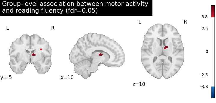
We compute the fdr-corrected p = 0.05 threshold for these data.
from nilearn.glm import threshold_stats_img

_, threshold = threshold_stats_img(z_map, alpha=0.05, height_control="fdr")
Let us plot the second level contrast at the computed thresholds.
from nilearn.plotting import plot_stat_map, show

cut_coords = [10, -5, 10]

plot_stat_map(
    z_map,
    threshold=threshold,
    title="Group-level association between motor activity \n"
    "and reading fluency (fdr=0.05)",
    cut_coords=cut_coords,
    draw_cross=False,
)

show()

Computing the (corrected) p-values with parametric test to compare with non parametric test
from nilearn.image import get_data, math_img

p_val = model.compute_contrast("fluency", output_type="p_value")
n_voxels = np.sum(get_data(model.mask_img_))
# Correcting the p-values for multiple testing and taking negative logarithm
neg_log_pval = math_img(
    f"-np.log10(np.minimum(1, img * {n_voxels!s}))", img=p_val
)
<string>:1: RuntimeWarning:

divide by zero encountered in log10
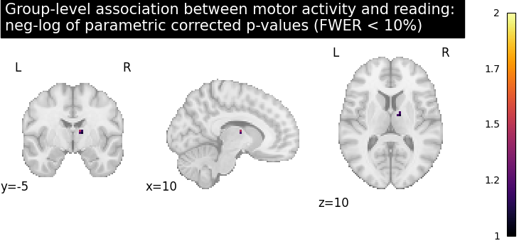
Let us plot the (corrected) negative log p-values for the parametric test
# Since we are plotting negative log p-values and using a threshold equal to 1,
# it corresponds to corrected p-values lower than 10%, meaning that there
# is less than 10% probability to make a single false discovery
# (90% chance that we make no false discoveries at all).
# This threshold is much more conservative than the previous one.
threshold = 1
title = (
    "Group-level association between motor activity and reading: \n"
    "neg-log of parametric corrected p-values (FWER < 10%)"
)
plot_stat_map(
    neg_log_pval,
    cut_coords=cut_coords,
    threshold=threshold,
    title=title,
    vmin=threshold,
    cmap="inferno",
    draw_cross=False,
)
show()

/home/runner/work/nilearn/nilearn/examples/05_glm_second_level/plot_second_level_association_test.py:119: UserWarning:

Non-finite values detected. These values will be replaced with zeros.
Computing the (corrected) negative log p-values with permutation test
from nilearn.glm.second_level import non_parametric_inference

neg_log_pvals_permuted_ols_unmasked = non_parametric_inference(
    contrast_map_filenames,
    design_matrix=design_matrix,
    second_level_contrast="fluency",
    model_intercept=True,
    n_perm=1000,
    two_sided_test=False,
    mask=None,
    smoothing_fwhm=5.0,
    n_jobs=2,
    verbose=1,
)
[non_parametric_inference] Fitting second level model...
[non_parametric_inference]
Computation of second level model done in 00 HR 00 MIN 00 SEC
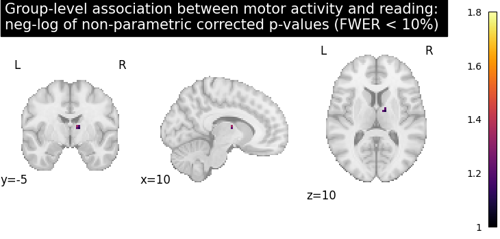
Let us plot the (corrected) negative log p-values
title = (
    "Group-level association between motor activity and reading: \n"
    "neg-log of non-parametric corrected p-values (FWER < 10%)"
)
plot_stat_map(
    neg_log_pvals_permuted_ols_unmasked,
    cut_coords=cut_coords,
    threshold=threshold,
    title=title,
    vmin=threshold,
    cmap="inferno",
    draw_cross=False,
)
show()

# The neg-log p-values obtained with non parametric testing are capped at 3
# since the number of permutations is 1e3.
# The non parametric test yields a few more discoveries
# and is then more powerful than the usual parametric procedure.

Total running time of the script: (3 minutes 36.817 seconds)
Estimated memory usage: 267 MB