Note
Go to the end to download the full example code. or to run this example in your browser via Binder
Seed-based connectivity on the surface
Warning
This is an adaption of Seed-based connectivity on the surface to use make it work with the new experimental surface API.
The dataset that is a subset of the enhanced NKI Rockland sample (https://fcon_1000.projects.nitrc.org/indi/enhanced/, Nooner et al.[1] see NKI enhanced surface dataset)
Resting state fMRI scans (TR=645ms) of 102 subjects were preprocessed (https://github.com/fliem/nki_nilearn) and projected onto the Freesurfer fsaverage5 template (Dale et al.[2] and Fischl et al.[3]). For this example we use the time series of a single subject’s left hemisphere.
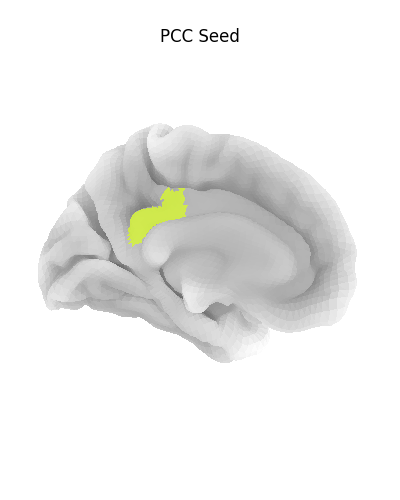
The Destrieux parcellation (Destrieux et al.[4]) in fsaverage5 space as distributed with Freesurfer is used to select a seed region in the posterior cingulate cortex.
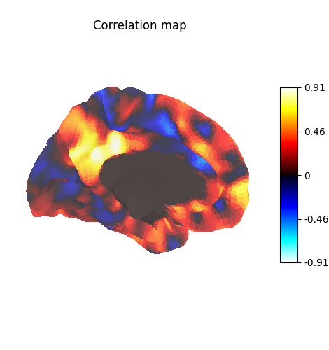
Functional connectivity of the seed region to all other cortical nodes in the same hemisphere is calculated using Pearson product-moment correlation coefficient.
The nilearn.plotting.plot_surf_stat_map function is used
to plot the resulting statistical map on the (inflated) pial surface.
See also for a similar example but using volumetric input data.
See Plotting brain images for more details on plotting tools.
Retrieving the data
# NKI resting state data from nilearn
from nilearn.experimental.surface import (
    fetch_destrieux,
    fetch_nki,
    load_fsaverage,
    load_fsaverage_data,
)

nki_dataset = fetch_nki(n_subjects=1)

# For this example we will only work on the data
# from the left hemisphere
hemi = "left"

# The nki list contains a SurfaceImage instance
# for the data of each subject along with fsaverage pial meshes.

# Destrieux parcellation for left hemisphere in fsaverage5 space
destrieux_atlas, labels = fetch_destrieux()
parcellation = destrieux_atlas.data.parts[hemi]

# Fsaverage5 surface template
fsaverage_meshes = load_fsaverage()

# The fsaverage meshes contains the FileMesh objects:
print(
    "Fsaverage5 pial surface of left hemisphere is: "
    f"{fsaverage_meshes['pial'].parts[hemi]}"
)
print(
    "Fsaverage5 inflated surface of left hemisphere is: "
    f"{fsaverage_meshes['flat'].parts[hemi]}"
)
print(
    "Fsaverage5 inflated surface of left hemisphere is: "
    f"{fsaverage_meshes['inflated'].parts[hemi]}"
)

# The fsaverage data contains SurfaceImage instances with meshes and data
fsaverage_sulcal = load_fsaverage_data(data_type="sulcal")
print(f"Fsaverage5 sulcal depth map: {fsaverage_sulcal}")

fsaverage_curvature = load_fsaverage_data(data_type="curvature")
print(f"Fsaverage5 sulcal curvature map: {fsaverage_curvature}")
[get_dataset_dir] Dataset found in /home/runner/work/nilearn/nilearn/nilearn_data/nki_enhanced_surface
[get_dataset_dir] Dataset found in /home/runner/work/nilearn/nilearn/nilearn_data/destrieux_surface
Fsaverage5 pial surface of left hemisphere is: <FileMesh with 10242 vertices>
Fsaverage5 inflated surface of left hemisphere is: <FileMesh with 10242 vertices>
Fsaverage5 inflated surface of left hemisphere is: <FileMesh with 10242 vertices>
Fsaverage5 sulcal depth map: <SurfaceImage (20484,)>
Fsaverage5 sulcal curvature map: <SurfaceImage (20484,)>
Extracting the seed time series
# Load resting state time series from nilearn
timeseries = nki_dataset[0].data.parts[hemi].T

# Coercing to float is required to avoid errors withj scipy >= 0.14.0
timeseries = timeseries.astype(float)

# Extract seed region via label
pcc_region = "G_cingul-Post-dorsal"

import numpy as np

pcc_labels = np.where(parcellation == labels.index(pcc_region))[0]

# Extract time series from seed region
seed_timeseries = np.mean(timeseries[pcc_labels], axis=0)
Calculating seed-based functional connectivity
# Calculate Pearson product-moment correlation coefficient between seed
# time series and timeseries of all cortical nodes of the hemisphere
from scipy import stats

stat_map = np.zeros(timeseries.shape[0])
for i in range(timeseries.shape[0]):
    stat_map[i] = stats.pearsonr(seed_timeseries, timeseries[i])[0]

# Re-mask previously masked nodes (medial wall)
stat_map[np.where(np.mean(timeseries, axis=1) == 0)] = 0
/home/runner/work/nilearn/nilearn/examples/08_experimental/plot_surf_stat_map_experimental.py:117: ConstantInputWarning:

An input array is constant; the correlation coefficient is not defined.
Display ROI on surface
# Transform ROI indices in ROI map
pcc_map = np.zeros(parcellation.shape[0], dtype=int)
pcc_map[pcc_labels] = 1

from nilearn.experimental import plotting
from nilearn.plotting import show

plotting.plot_surf_roi(
    surf_mesh=nki_dataset[0].mesh,
    roi_map=pcc_map,
    hemi=hemi,
    view="medial",
    bg_map=fsaverage_sulcal,
    bg_on_data=True,
    title="PCC Seed",
)

show()
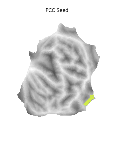
Using a flat mesh can be useful in order to easily locate the area of interest on the cortex. To make this plot easier to read, we use the mesh curvature as a background map.
bg_map = np.sign(fsaverage_curvature.data.parts[hemi])
# np.sign yields values in [-1, 1]. We rescale the background map
# such that values are in [0.25, 0.75], resulting in a nicer looking plot.
bg_map_rescaled = (bg_map + 1) / 4 + 0.25

plotting.plot_surf_roi(
    surf_mesh=fsaverage_meshes["flat"],
    roi_map=pcc_map,
    hemi=hemi,
    view="dorsal",
    bg_map=fsaverage_sulcal,
    bg_on_data=True,
    title="PCC Seed",
)
<Figure size 400x500 with 1 Axes>
Display unthresholded stat map with a slightly dimmed background
plotting.plot_surf_stat_map(
    surf_mesh=nki_dataset[0].mesh,
    stat_map=stat_map,
    hemi=hemi,
    view="medial",
    colorbar=True,
    bg_map=fsaverage_sulcal,
    bg_on_data=True,
    darkness=0.3,
    title="Correlation map",
)

show()
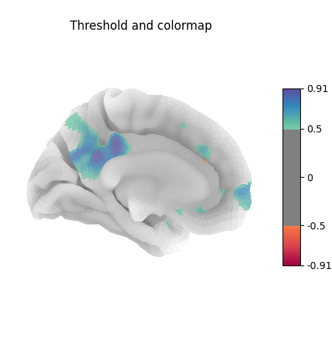
Many different options are available for plotting, for example thresholding, or using custom colormaps
plotting.plot_surf_stat_map(
    surf_mesh=nki_dataset[0].mesh,
    stat_map=stat_map,
    hemi=hemi,
    view="medial",
    colorbar=True,
    bg_map=fsaverage_sulcal,
    bg_on_data=True,
    cmap="Spectral",
    threshold=0.5,
    title="Threshold and colormap",
)

show()
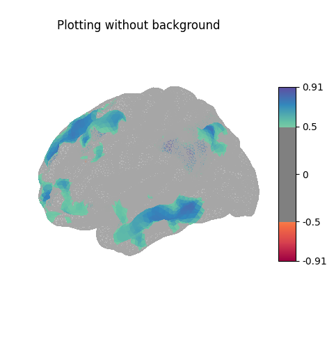
Here the surface is plotted in a lateral view without a background map. To capture 3D structure without depth information, the default is to plot a half transparent surface. Note that you can also control the transparency with a background map using the alpha parameter.
plotting.plot_surf_stat_map(
    surf_mesh=nki_dataset[0].mesh,
    stat_map=stat_map,
    hemi=hemi,
    view="lateral",
    colorbar=True,
    cmap="Spectral",
    threshold=0.5,
    title="Plotting without background",
)

show()
The plots can be saved to file, in which case the display is closed after creating the figure
from pathlib import Path

output_dir = Path.cwd() / "results" / "plot_surf_stat_map"
output_dir.mkdir(exist_ok=True, parents=True)
print(f"Output will be saved to: {output_dir}")

plotting.plot_surf_stat_map(
    surf_mesh=fsaverage_meshes["inflated"],
    stat_map=stat_map,
    hemi=hemi,
    bg_map=fsaverage_sulcal,
    bg_on_data=True,
    threshold=0.5,
    colorbar=True,
    output_file=output_dir / "plot_surf_stat_map.png",
)

show()
Output will be saved to: /home/runner/work/nilearn/nilearn/examples/08_experimental/results/plot_surf_stat_map
References
Total running time of the script: (0 minutes 23.618 seconds)
Estimated memory usage: 935 MB