Example of surface-based first-level analysis

Warning

This example is adapted from Example of surface-based first-level analysis. # noqa to show how to use the new tentative API for surface images in nilearn.

This functionality is provided by the nilearn.experimental.surface module.

It is still incomplete and subject to change without a deprecation cycle.

Please participate in the discussion on GitHub!

A full step-by-step example of fitting a GLM to experimental data sampled on the cortical surface and visualizing the results.

More specifically:

1. A sequence of fMRI volumes is loaded.

2. fMRI data are projected onto a reference cortical surface (the FreeSurfer template, fsaverage).

3. A GLM is applied to the dataset (effect/covariance, then contrast estimation).

The result of the analysis are statistical maps that are defined on the brain mesh. We display them using Nilearn capabilities.

The projection of fMRI data onto a given brain mesh requires that both are initially defined in the same space.

• The functional data should be coregistered to the anatomy from which the mesh was obtained.

• Another possibility, used here, is to project the normalized fMRI data to an MNI-coregistered mesh, such as fsaverage.

The advantage of this second approach is that it makes it easy to run second-level analyses on the surface. On the other hand, it is obviously less accurate than using a subject-tailored mesh.

Prepare data and analysis parameters

Prepare the timing parameters.

t_r = 2.4
slice_time_ref = 0.5

Prepare the data. First, the volume-based fMRI data.

from nilearn import datasets

data = datasets.fetch_localizer_first_level()
fmri_img = data.epi_img

[get_dataset_dir] Dataset found in /home/runner/work/nilearn/nilearn/nilearn_data/localizer_first_level

Second, the experimental paradigm.

import pandas as pd

events_file = data.events
events = pd.read_table(events_file)

Project the fMRI image to the surface

For this we need to get a mesh representing the geometry of the surface. We could use an individual mesh, but we first resort to a standard mesh, the so-called fsaverage5 template from the FreeSurfer software.

We use the new nilearn.experimental.surface.SurfaceImage to create an surface object instance that contains both the mesh (here we use the one from the fsaverage5 templates) and the BOLD data that we project on the surface.

from nilearn.experimental.surface import SurfaceImage, load_fsaverage

fsaverage5 = load_fsaverage()
image = SurfaceImage(
    mesh=fsaverage5["pial"],
    data=fmri_img,
)

Perform first level analysis

We can now simply run a GLM by directly passing our nilearn.experimental.surface.SurfaceImage instance as input to FirstLevelModel.fit

Here we use an HRF model containing the Glover model and its time derivative The drift model is implicitly a cosine basis with a period cutoff at 128s.

from nilearn.glm.first_level import FirstLevelModel

glm = FirstLevelModel(
    t_r,
    slice_time_ref=slice_time_ref,
    hrf_model="glover + derivative",
).fit(image, events)

Estimate contrasts

Specify the contrasts.

For practical purpose, we first generate an identity matrix whose size is the number of columns of the design matrix.

import numpy as np

design_matrix = glm.design_matrices_[0]
contrast_matrix = np.eye(design_matrix.shape[1])

At first, we create basic contrasts.

basic_contrasts = {
    column: contrast_matrix[i]
    for i, column in enumerate(design_matrix.columns)
}

Next, we add some intermediate contrasts and one contrast adding all conditions with some auditory parts.

basic_contrasts["audio"] = (
    basic_contrasts["audio_left_hand_button_press"]
    + basic_contrasts["audio_right_hand_button_press"]
    + basic_contrasts["audio_computation"]
    + basic_contrasts["sentence_listening"]
)

# one contrast adding all conditions involving instructions reading
basic_contrasts["visual"] = (
    basic_contrasts["visual_left_hand_button_press"]
    + basic_contrasts["visual_right_hand_button_press"]
    + basic_contrasts["visual_computation"]
    + basic_contrasts["sentence_reading"]
)

# one contrast adding all conditions involving computation
basic_contrasts["computation"] = (
    basic_contrasts["visual_computation"]
    + basic_contrasts["audio_computation"]
)

# one contrast adding all conditions involving sentences
basic_contrasts["sentences"] = (
    basic_contrasts["sentence_listening"] + basic_contrasts["sentence_reading"]
)

Finally, we create a dictionary of more relevant contrasts

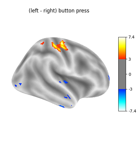
• ‘left - right button press’: probes motor activity in left versus right button presses.

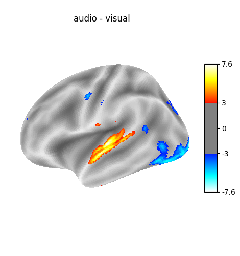
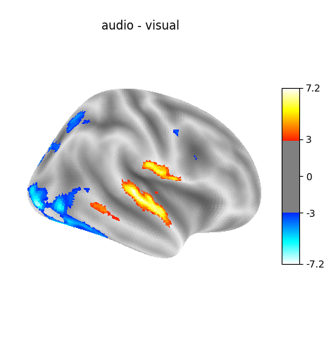
• ‘audio - visual’: probes the difference of activity between listening to some content or reading the same type of content (instructions, stories).

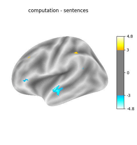
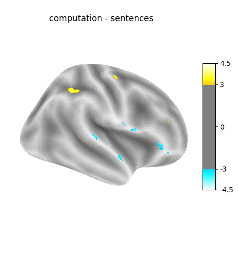
• ‘computation - sentences’: looks at the activity when performing a mental computation task versus simply reading sentences.

Of course, we could define other contrasts, but we keep only 3 for simplicity.

contrasts = {
    "(left - right) button press": (
        basic_contrasts["audio_left_hand_button_press"]
        - basic_contrasts["audio_right_hand_button_press"]
        + basic_contrasts["visual_left_hand_button_press"]
        - basic_contrasts["visual_right_hand_button_press"]
    ),
    "audio - visual": basic_contrasts["audio"] - basic_contrasts["visual"],
    "computation - sentences": (
        basic_contrasts["computation"] - basic_contrasts["sentences"]
    ),
}


from nilearn.experimental.plotting import plot_surf_stat_map
from nilearn.experimental.surface import load_fsaverage_data

Let’s estimate the contrasts by iterating over them.

from nilearn.plotting import show

fsaverage_data = load_fsaverage_data(data_type="sulcal")

for index, (contrast_id, contrast_val) in enumerate(contrasts.items()):
    # compute contrast-related statistics
    z_score = glm.compute_contrast(contrast_val, stat_type="t")

    # we plot it on the surface, on the inflated fsaverage mesh,
    # together with a suitable background to give an impression
    # of the cortex folding.
    for hemi in ["left", "right"]:
        print(
            f"  Contrast {index + 1:1} out of {len(contrasts)}: "
            f"{contrast_id}, {hemi} hemisphere"
        )
        plot_surf_stat_map(
            surf_mesh=fsaverage5["inflated"],
            stat_map=z_score,
            hemi=hemi,
            title=contrast_id,
            colorbar=True,
            threshold=3.0,
            bg_map=fsaverage_data,
        )

show()

• 
• 
• 
• 
• 
• 

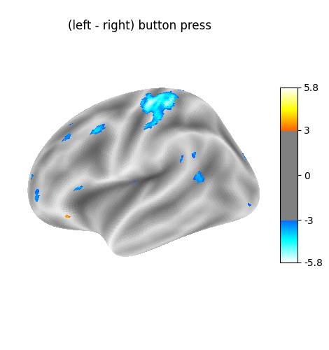
Contrast 1 out of 3: (left - right) button press, left hemisphere
Contrast 1 out of 3: (left - right) button press, right hemisphere
Contrast 2 out of 3: audio - visual, left hemisphere
Contrast 2 out of 3: audio - visual, right hemisphere
Contrast 3 out of 3: computation - sentences, left hemisphere
Contrast 3 out of 3: computation - sentences, right hemisphere

Estimated memory usage: 370 MB