Surface-based dataset first and second level analysis of a dataset

Warning

This example is adapted from Surface-based dataset first and second level analysis of a dataset. to show how to use the new tentative API for surface images in nilearn.

This functionality is provided by the nilearn.experimental.surface module.

It is still incomplete and subject to change without a deprecation cycle.

Please participate in the discussion on GitHub!

Full step-by-step example of fitting a GLM (first and second level analysis) in a 10-subjects dataset and visualizing the results.

More specifically:

1. Download an fMRI BIDS dataset with two language conditions to contrast.

2. Project the data to a standard mesh, fsaverage5, also known as the Freesurfer template mesh downsampled to about 10k nodes per hemisphere.

3. Run the first level model objects.

4. Fit a second level model on the fitted first level models.

Notice that in this case the preprocessed bold images were already normalized to the same MNI space.

from nilearn._utils.helpers import check_matplotlib

check_matplotlib()

Fetch example BIDS dataset

We download a simplified BIDS dataset made available for illustrative purposes. It contains only the necessary information to run a statistical analysis using Nilearn. The raw data subject folders only contain bold.json and events.tsv files, while the derivatives folder includes the preprocessed files preproc.nii and the confounds.tsv files.

from nilearn.datasets import fetch_language_localizer_demo_dataset

data = fetch_language_localizer_demo_dataset(legacy_output=False)

[get_dataset_dir] Dataset found in /home/runner/work/nilearn/nilearn/nilearn_data/fMRI-language-localizer-demo-dataset

Here is the location of the dataset on disk.

print(data.data_dir)

/home/runner/work/nilearn/nilearn/nilearn_data/fMRI-language-localizer-demo-dataset

Obtain automatically FirstLevelModel objects and fit arguments

From the dataset directory we automatically obtain the FirstLevelModel objects with their subject_id filled from the BIDS dataset. Moreover, we obtain for each model a dictionary with run_imgs, events and confounder regressors since in this case a confounds.tsv file is available in the BIDS dataset. To get the first level models we only have to specify the dataset directory and the task_label as specified in the file names.

from nilearn.glm.first_level import first_level_from_bids

task_label = "languagelocalizer"
models, run_imgs, events, confounds = first_level_from_bids(
    data.data_dir,
    task_label,
    img_filters=[("desc", "preproc")],
    hrf_model="glover + derivative",
    n_jobs=2,
)

/home/runner/work/nilearn/nilearn/examples/08_experimental/plot_new_surface_bids_analysis_experimental.py:76: UserWarning:

'StartTime' not found in file /home/runner/work/nilearn/nilearn/nilearn_data/fMRI-language-localizer-demo-dataset/derivatives/sub-01/func/sub-01_task-languagelocalizer_desc-preproc_bold.json.

Project fMRI data to the surface and compute GLM and contrasts

The projection function simply takes the fMRI data and the mesh. Note that those correspond spatially, as they are both in MNI space.

from pathlib import Path

from nilearn.experimental.surface import SurfaceImage, load_fsaverage

fsaverage5 = load_fsaverage()

# Empty lists in which we are going to store activation values.
z_scores_left = []
z_scores_right = []
for first_level_glm, fmri_img, confound, event in zip(
    models, run_imgs, confounds, events
):
    print(f"Running GLM on {Path(fmri_img[0]).relative_to(data.data_dir)}")

    image = SurfaceImage.from_volume(
        mesh=fsaverage5["pial"],
        volume_img=fmri_img[0],
    )

    # Fit GLM.
    first_level_glm.fit(run_imgs=image, events=event[0], confounds=confound[0])

    # Contrast specification
    design_matrix = first_level_glm.design_matrices_[0]
    contrast_values = (design_matrix.columns == "language") * 1.0 - (
        design_matrix.columns == "string"
    )
    z_scores = first_level_glm.compute_contrast(contrast_values, stat_type="t")
    z_scores_left.append(z_scores.data.parts["left"])
    z_scores_right.append(z_scores.data.parts["right"])

Running GLM on derivatives/sub-01/func/sub-01_task-languagelocalizer_desc-preproc_bold.nii.gz
Running GLM on derivatives/sub-02/func/sub-02_task-languagelocalizer_desc-preproc_bold.nii.gz
Running GLM on derivatives/sub-03/func/sub-03_task-languagelocalizer_desc-preproc_bold.nii.gz
Running GLM on derivatives/sub-04/func/sub-04_task-languagelocalizer_desc-preproc_bold.nii.gz
Running GLM on derivatives/sub-05/func/sub-05_task-languagelocalizer_desc-preproc_bold.nii.gz
Running GLM on derivatives/sub-06/func/sub-06_task-languagelocalizer_desc-preproc_bold.nii.gz
Running GLM on derivatives/sub-07/func/sub-07_task-languagelocalizer_desc-preproc_bold.nii.gz
Running GLM on derivatives/sub-08/func/sub-08_task-languagelocalizer_desc-preproc_bold.nii.gz
Running GLM on derivatives/sub-09/func/sub-09_task-languagelocalizer_desc-preproc_bold.nii.gz
Running GLM on derivatives/sub-10/func/sub-10_task-languagelocalizer_desc-preproc_bold.nii.gz

Group study

Individual activation maps have been accumulated in the z_score_left and z_scores_right lists respectively. We can now use them in a group study (one-sample study).

Prepare figure for concurrent plot of individual maps compute population-level maps for left and right hemisphere We directly do that on the value arrays.

import numpy as np
from scipy.stats import norm, ttest_1samp

_, pval_left = ttest_1samp(np.array(z_scores_left), 0)
_, pval_right = ttest_1samp(np.array(z_scores_right), 0)

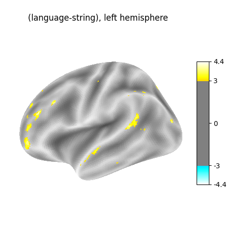
What we have so far are p-values: we convert them to z-values for plotting.

z_val_left = norm.isf(pval_left)
z_val_right = norm.isf(pval_right)

Plot the resulting maps, at first on the left hemisphere.

from nilearn.experimental.plotting import plot_surf_stat_map
from nilearn.experimental.surface import load_fsaverage_data
from nilearn.plotting import show

fsaverage_data = load_fsaverage_data(data_type="sulcal")

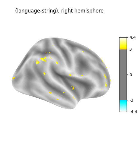
for hemi, stat_map in zip(["left", "right"], [z_val_left, z_val_right]):
    plot_surf_stat_map(
        surf_mesh=fsaverage5["inflated"],
        stat_map=stat_map,
        hemi=hemi,
        title=f"(language-string), {hemi} hemisphere",
        colorbar=True,
        threshold=3.0,
        bg_map=fsaverage_data,
    )

show()

• 
• 

Estimated memory usage: 956 MB