Making a surface plot of a 3D statistical map

Warning

This is an adaption of Making a surface plot of a 3D statistical map to use make it work with the new experimental surface API.

In this example, we will project a 3D statistical map onto a cortical mesh using vol_to_surf, display a surface plot of the projected map using plot_surf_stat_map with different plotting engines, and add contours of regions of interest using plot_surf_contours.

Get a statistical map

from nilearn import datasets

stat_img = datasets.load_sample_motor_activation_image()

Get a cortical mesh

from nilearn.experimental.surface import load_fsaverage, load_fsaverage_data

fsaverage_meshes = load_fsaverage()

Use mesh curvature to display useful anatomical information on inflated meshes

Here, we load the curvature map of the hemisphere under study, and define a surface map whose value for a given vertex is 1 if the curvature is positive, -1 if the curvature is negative.

import numpy as np

fsaverage_curvature = load_fsaverage_data(data_type="curvature")
curv_right_sign = np.sign(fsaverage_curvature.data.parts["right"])

Sample the 3D data around each node of the mesh

from nilearn.experimental.surface import SurfaceImage

img = SurfaceImage(
    mesh=fsaverage_meshes["pial"],
    data=stat_img,
)

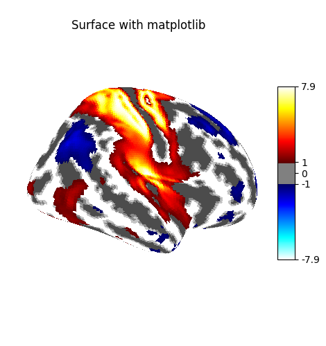
Plot the result

You can visualize the texture on the surface using the function plot_surf_stat_map which uses matplotlib as the default plotting engine.

from nilearn.experimental.plotting import plot_surf_stat_map

fig = plot_surf_stat_map(
    stat_map=img,
    surf_mesh=fsaverage_meshes["inflated"],
    hemi="right",
    title="Surface with matplotlib",
    colorbar=True,
    threshold=1.0,
    bg_map=curv_right_sign,
)
fig.show()

Interactive plotting with Plotly

If you have a recent version of Nilearn (>=0.8.2), and if you have plotly installed, you can easily configure plot_surf_stat_map to use plotly instead of matplotlib:

engine = "plotly"
# If plotly is not installed, use matplotlib
try:
    import plotly.graph_objects as go  # noqa: F401
except ImportError:
    engine = "matplotlib"

print(f"Using plotting engine {engine}.")

fig = plot_surf_stat_map(
    stat_map=img,
    surf_mesh=fsaverage_meshes["inflated"],
    hemi="right",
    title="Surface with plotly",
    colorbar=True,
    threshold=1.0,
    bg_map=curv_right_sign,
    bg_on_data=True,
    engine=engine,  # Specify the plotting engine here
)

# Display the figure as with matplotlib figures
# fig.show()

Using plotting engine plotly.
/opt/hostedtoolcache/Python/3.12.5/x64/lib/python3.12/site-packages/nilearn/plotting/surf_plotting.py:980: UserWarning:

vmin cannot be chosen when cmap is symmetric

When using matplolib as the plotting engine, a standard matplotlib.figure.Figure is returned. With plotly as the plotting engine, a custom PlotlySurfaceFigure is returned which provides a similar API to the Figure. For example, you can save a static version of the figure to file (this option requires to have kaleido installed):

# Save the figure as we would do with a matplotlib figure.
# Uncomment the following line to save the previous figure to file
# fig.savefig("right_hemisphere.png")

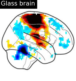
Plot 3D image for comparison

from nilearn import plotting

plotting.plot_glass_brain(
    stat_map_img=stat_img,
    display_mode="r",
    plot_abs=False,
    title="Glass brain",
    threshold=2.0,
)

plotting.plot_stat_map(
    stat_map_img=stat_img,
    display_mode="x",
    threshold=1.0,
    cut_coords=range(0, 51, 10),
    title="Slices",
)

• 
• 

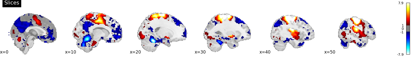
<nilearn.plotting.displays._slicers.XSlicer object at 0x7fdeeda65ca0>

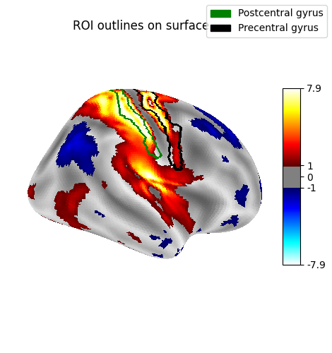
Use an atlas and choose regions to outline

from nilearn.experimental.surface import fetch_destrieux

destrieux_atlas, label_names = fetch_destrieux(mesh_type="inflated")

# these are the regions we want to outline
regions_dict = {
    "G_postcentral": "Postcentral gyrus",
    "G_precentral": "Precentral gyrus",
}

# get indices in atlas for these labels
regions_indices = [
    np.where(np.array(label_names) == region)[0][0] for region in regions_dict
]

labels = list(regions_dict.values())

[get_dataset_dir] Dataset found in /home/runner/work/nilearn/nilearn/nilearn_data/destrieux_surface

Display outlines of the regions of interest on top of a statistical map

from nilearn.experimental.plotting import plot_surf_contours

fsaverage_sulcal = load_fsaverage_data(data_type="sulcal", mesh_type="pial")

figure = plot_surf_stat_map(
    stat_map=img,
    surf_mesh=fsaverage_meshes["inflated"],
    hemi="right",
    title="ROI outlines on surface",
    colorbar=True,
    threshold=1.0,
    bg_map=fsaverage_sulcal,
)

plot_surf_contours(
    roi_map=destrieux_atlas,
    hemi="right",
    labels=labels,
    levels=regions_indices,
    figure=figure,
    legend=True,
    colors=["g", "k"],
)
plotting.show()

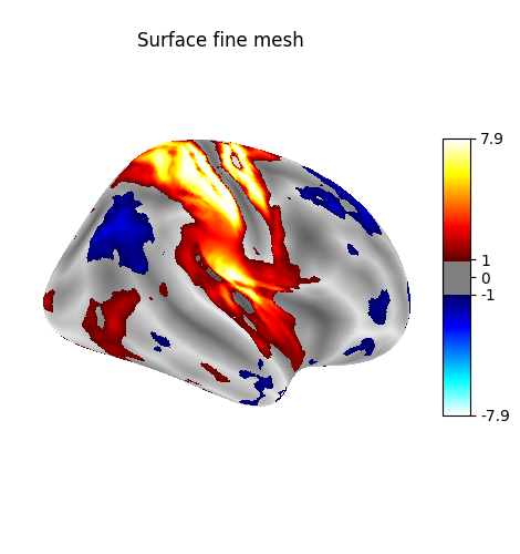
Plot with higher-resolution mesh

fetch_surf_fsaverage takes a mesh argument which specifies whether to fetch the low-resolution fsaverage5 mesh, or the high-resolution fsaverage mesh. Using mesh="fsaverage" will result in more memory usage and computation time, but finer visualizations.

big_fsaverage_meshes = load_fsaverage("fsaverage")

big_fsaverage_sulcal = load_fsaverage_data(
    mesh_name="fsaverage", data_type="sulcal", mesh_type="inflated"
)

big_img = SurfaceImage(
    mesh=big_fsaverage_meshes["pial"],
    data=stat_img,
)

plot_surf_stat_map(
    big_img,
    surf_mesh=big_fsaverage_meshes["inflated"],
    hemi="right",
    colorbar=True,
    title="Surface fine mesh",
    threshold=1.0,
    bg_map=big_fsaverage_sulcal,
)

[get_dataset_dir] Dataset found in /home/runner/work/nilearn/nilearn/nilearn_data/fsaverage
[get_dataset_dir] Dataset found in /home/runner/work/nilearn/nilearn/nilearn_data/fsaverage
[get_dataset_dir] Dataset found in /home/runner/work/nilearn/nilearn/nilearn_data/fsaverage

<Figure size 470x500 with 2 Axes>

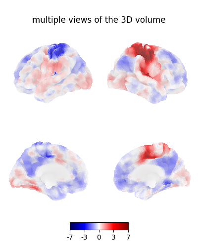
Plot multiple views of the 3D volume on a surface

plot_img_on_surf takes a statistical map and projects it onto a surface. It supports multiple choices of orientations, and can plot either one or both hemispheres. If no surf_mesh is given, plot_img_on_surf projects the images onto FreeSurfer's fsaverage5.

plotting.plot_img_on_surf(
    stat_img,
    views=["lateral", "medial"],
    hemispheres=["left", "right"],
    colorbar=True,
    cmap="seismic",
    title="multiple views of the 3D volume",
    bg_on_data=True,
)
plotting.show()

3D visualization in a web browser

An alternative to nilearn.plotting.plot_surf_stat_map is to use nilearn.plotting.view_surf or nilearn.plotting.view_img_on_surf that give more interactive visualizations in a web browser. See 3D Plots of statistical maps or atlases on the cortical surface for more details.

from nilearn.experimental.plotting import view_surf

view = view_surf(
    surf_mesh=fsaverage_meshes["inflated"],
    surf_map=img,
    threshold="90%",
    bg_map=fsaverage_sulcal,
    hemi="right",
    title="3D visualization in a web browser",
)

# In a Jupyter notebook, if ``view`` is the output of a cell,
# it will be displayed below the cell
view
# view.open_in_browser()

# We don't need to do the projection ourselves, we can use
# :func:`~nilearn.plotting.view_img_on_surf`:

view = plotting.view_img_on_surf(stat_img, threshold="90%")

view
# view.open_in_browser()

Impact of plot parameters on visualization

You can specify arguments to be passed on to the function nilearn.surface.vol_to_surf using vol_to_surf_kwargs This allows fine-grained control of how the input 3D image is resampled and interpolated - for example if you are viewing a volumetric atlas, you would want to avoid averaging the labels between neighboring regions. Using nearest-neighbor interpolation with zero radius will achieve this.

destrieux = datasets.fetch_atlas_destrieux_2009(legacy_format=False)

view = plotting.view_img_on_surf(
    destrieux.maps,
    surf_mesh="fsaverage",
    cmap="tab20",
    vol_to_surf_kwargs={
        "n_samples": 1,
        "radius": 0.0,
        "interpolation": "nearest",
    },
    symmetric_cmap=False,
    colorbar=False,
)

view
# view.open_in_browser()

[get_dataset_dir] Dataset found in /home/runner/work/nilearn/nilearn/nilearn_data/destrieux_2009
[get_dataset_dir] Dataset found in /home/runner/work/nilearn/nilearn/nilearn_data/fsaverage

Estimated memory usage: 670 MB