Note

Go to the end to download the full example code or to run this example in your browser via Binder

Advanced decoding using scikit learn#

This tutorial opens the box of decoding pipelines to bridge integrated functionalities provided by the nilearn.decoding.Decoder object with more advanced usecases. It reproduces basic examples functionalities with direct calls to scikit-learn function and gives pointers to more advanced objects. If some concepts seem unclear, please refer to the documentation on decoding and in particular to the advanced section. As in many other examples, we perform decoding of the visual category of a stimuli on Haxby et al.[1] dataset, focusing on distinguishing two categories: face and cat images.

Note

If you are using Nilearn with a version older than 0.9.0, then you should either upgrade your version or import maskers from the input_data module instead of the maskers module.

That is, you should manually replace in the following example all occurrences of:

from nilearn.maskers import NiftiMasker

with:

from nilearn.input_data import NiftiMasker

Retrieve and load the fMRI data from the Haxby study#

First download the data#

# The :func:`nilearn.datasets.fetch_haxby` function will download the
# Haxby dataset composed of fMRI images in a Niimg,
# a spatial mask and a text document with label of each image
from nilearn import datasets

haxby_dataset = datasets.fetch_haxby()
mask_filename = haxby_dataset.mask_vt[0]
fmri_filename = haxby_dataset.func[0]

# Loading the behavioral labels
import pandas as pd

behavioral = pd.read_csv(haxby_dataset.session_target[0], delimiter=" ")
behavioral

	labels	chunks
0	rest	0
1	rest	0
2	rest	0
3	rest	0
4	rest	0
...	...	...
1447	rest	11
1448	rest	11
1449	rest	11
1450	rest	11
1451	rest	11

1452 rows × 2 columns

We keep only a images from a pair of conditions(cats versus faces).

from nilearn.image import index_img

conditions = behavioral["labels"]
condition_mask = conditions.isin(["face", "cat"])
fmri_niimgs = index_img(fmri_filename, condition_mask)
conditions = conditions[condition_mask]
# Convert to numpy array
conditions = conditions.values
run_label = behavioral["chunks"][condition_mask]

Performing decoding with scikit-learn#

# Importing a classifier
# ......................
# We can import many predictive models from scikit-learn that can be used in a
# decoding pipelines. They are all used with the same `fit()` and `predict()`
# functions.
# Let's define a Support Vector Classifier
# (or `SVC <https://scikit-learn.org/stable/modules/svm.html >`_).

from sklearn.svm import SVC

svc = SVC()

Masking the data#

To use a scikit-learn estimator on brain images, you should first mask the data using a nilearn.maskers.NiftiMasker to extract only the voxels inside the mask of interest, and transform 4D input fMRI data to 2D arrays (shape=(n_timepoints, n_voxels)) that estimators can work on.

from nilearn.maskers import NiftiMasker

masker = NiftiMasker(
    mask_img=mask_filename,
    runs=run_label,
    smoothing_fwhm=4,
    standardize="zscore_sample",
    memory="nilearn_cache",
    memory_level=1,
)
fmri_masked = masker.fit_transform(fmri_niimgs)

/home/himanshu/Desktop/nilearn_work/nilearn/nilearn/image/resampling.py:492: UserWarning: The provided image has no sform in its header. Please check the provided file. Results may not be as expected.
  warnings.warn(

Cross-validation with scikit-learn#

To train and test the model in a meaningful way we use cross-validation with the function sklearn.model_selection.cross_val_score that computes for you the score for the different folds of cross-validation.

from sklearn.model_selection import cross_val_score

# Here `cv=5` stipulates a 5-fold cross-validation
cv_scores = cross_val_score(svc, fmri_masked, conditions, cv=5)
print(f"SVC accuracy: {cv_scores.mean():.3f}")

SVC accuracy: 0.823

Tuning cross-validation parameters#

You can change many parameters of the cross_validation here, for example:

use a different cross - validation scheme, for example LeaveOneGroupOut()
speed up the computation by using n_jobs = -1, which will spread the computation equally across all processors.
use a different scoring function, as a keyword or imported from scikit-learn : scoring = ‘roc_auc’

from sklearn.model_selection import LeaveOneGroupOut

cv = LeaveOneGroupOut()
cv_scores = cross_val_score(
    svc,
    fmri_masked,
    conditions,
    cv=cv,
    scoring="roc_auc",
    groups=run_label,
    n_jobs=2,
)
print(f"SVC accuracy (tuned parameters): {cv_scores.mean():.3f}")

SVC accuracy (tuned parameters): 0.858

Measuring the chance level#

sklearn.dummy.DummyClassifier (purely random) estimators are the simplest way to measure prediction performance at chance. A more controlled way, but slower, is to do permutation testing on the labels, with sklearn.model_selection.permutation_test_score.

Dummy estimator#

from sklearn.dummy import DummyClassifier

null_cv_scores = cross_val_score(
    DummyClassifier(), fmri_masked, conditions, cv=cv, groups=run_label
)

print(f"Dummy accuracy: {null_cv_scores.mean():.3f}")

Dummy accuracy: 0.500

Permutation test#

from sklearn.model_selection import permutation_test_score

null_cv_scores = permutation_test_score(
    svc, fmri_masked, conditions, cv=cv, groups=run_label
)[1]
print(f"Permutation test score: {null_cv_scores.mean():.3f}")

Permutation test score: 0.502

Decoding without a mask: Anova-SVM in scikit-lean#

We can also implement feature selection before decoding as a scikit-learn pipeline`(:class:`sklearn.pipeline.Pipeline). For this, we need to import the sklearn.feature_selection module and use sklearn.feature_selection.f_classif, a simple F-score based feature selection (a.k.a. Anova).

from sklearn.feature_selection import SelectPercentile, f_classif
from sklearn.pipeline import Pipeline
from sklearn.svm import LinearSVC

feature_selection = SelectPercentile(f_classif, percentile=10)
linear_svc = LinearSVC(dual=True)
anova_svc = Pipeline([("anova", feature_selection), ("svc", linear_svc)])

# We can use our ``anova_svc`` object exactly as we were using our ``svc``
# object previously.
# As we want to investigate our model, we use sklearn `cross_validate` function
# with `return_estimator = True` instead of cross_val_score,
# to save the estimator
from sklearn.model_selection import cross_validate

fitted_pipeline = cross_validate(
    anova_svc,
    fmri_masked,
    conditions,
    cv=cv,
    groups=run_label,
    return_estimator=True,
)
print(f"ANOVA+SVC test score: {fitted_pipeline['test_score'].mean():.3f}")

ANOVA+SVC test score: 0.801

Visualize the ANOVA + SVC’s discriminating weights#

# retrieve the pipeline fitted on the first cross-validation fold and its SVC
# coefficients
first_pipeline = fitted_pipeline["estimator"][0]
svc_coef = first_pipeline.named_steps["svc"].coef_
print(
    "After feature selection, "
    f"the SVC is trained only on {svc_coef.shape[1]} features"
)

# We invert the feature selection step to put these coefs in the right 2D place
full_coef = first_pipeline.named_steps["anova"].inverse_transform(svc_coef)

print(
    "After inverting feature selection, "
    f"we have {full_coef.shape[1]} features back"
)

# We apply the inverse of masking on these to make a 4D image that we can plot
from nilearn.plotting import plot_stat_map

weight_img = masker.inverse_transform(full_coef)
plot_stat_map(weight_img, title="Anova+SVC weights")

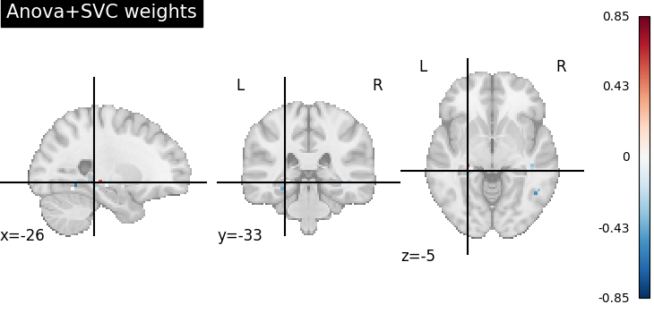
After feature selection, the SVC is trained only on 47 features
After inverting feature selection, we have 464 features back

<nilearn.plotting.displays._slicers.OrthoSlicer object at 0x7214eb7af110>

Going further with scikit-learn#

Changing the prediction engine#

To change the prediction engine, we just need to import it and use in our pipeline instead of the SVC. We can try Fisher’s Linear Discriminant Analysis (LDA) # noqa

# Construct the new estimator object and use it in a new pipeline after anova
from sklearn.discriminant_analysis import LinearDiscriminantAnalysis

feature_selection = SelectPercentile(f_classif, percentile=10)
lda = LinearDiscriminantAnalysis()
anova_lda = Pipeline([("anova", feature_selection), ("LDA", lda)])

# Recompute the cross-validation score:
import numpy as np

cv_scores = cross_val_score(
    anova_lda, fmri_masked, conditions, cv=cv, verbose=1, groups=run_label
)
classification_accuracy = np.mean(cv_scores)
n_conditions = len(set(conditions))  # number of target classes
print(
    "ANOVA + LDA classification accuracy: %.4f / Chance Level: %.4f"
    % (classification_accuracy, 1.0 / n_conditions)
)

ANOVA + LDA classification accuracy: 0.8009 / Chance Level: 0.5000

Changing the feature selection#

Let’s say that you want a more sophisticated feature selection, for example a Recursive Feature Elimination(RFE) before a svc. We follows the same principle.

# Import it and define your fancy objects
from sklearn.feature_selection import RFE

svc = SVC()
rfe = RFE(SVC(kernel="linear", C=1.0), n_features_to_select=50, step=0.25)

# Create a new pipeline, composing the two classifiers `rfe` and `svc`

rfe_svc = Pipeline([("rfe", rfe), ("svc", svc)])

# Recompute the cross-validation score
# cv_scores = cross_val_score(rfe_svc,
#                             fmri_masked,
#                             target,
#                             cv=cv,
#                             n_jobs=2,
#                             verbose=1)
# But, be aware that this can take * A WHILE * ...

References#

[1]
James V. Haxby, M. Ida Gobbini, Maura L. Furey, Alumit Ishai, Jennifer L. Schouten, and Pietro Pietrini. Distributed and overlapping representations of faces and objects in ventral temporal cortex. Science, 293(5539):2425–2430, 2001. URL: https://science.sciencemag.org/content/293/5539/2425, arXiv:https://science.sciencemag.org/content/293/5539/2425.full.pdf, doi:10.1126/science.1063736.

Total running time of the script: (0 minutes 19.913 seconds)

Estimated memory usage: 916 MB

Gallery generated by Sphinx-Gallery