Regions extraction using dictionary learning and functional connectomes

This example shows how to use nilearn.regions.RegionExtractor to extract spatially constrained brain regions from whole brain maps decomposed using Dictionary learning and use them to build a functional connectome.

We used 20 movie-watching functional datasets from nilearn.datasets.fetch_development_fmri and nilearn.decomposition.DictLearning for set of brain atlas maps.

This example can also be inspired to apply the same steps to even regions extraction using ICA maps. In that case, idea would be to replace Dictionary learning to canonical ICA decomposition using nilearn.decomposition.CanICA

Please see the related documentation of nilearn.regions.RegionExtractor for more details.

Fetch brain development functional datasets

We use nilearn’s datasets downloading utilities

from nilearn import datasets

rest_dataset = datasets.fetch_development_fmri(n_subjects=20)
func_filenames = rest_dataset.func
confounds = rest_dataset.confounds

[get_dataset_dir] Dataset found in /home/remi/nilearn_data/development_fmri
[get_dataset_dir] Dataset found in /home/remi/nilearn_data/development_fmri/development_fmri
[get_dataset_dir] Dataset found in /home/remi/nilearn_data/development_fmri/development_fmri

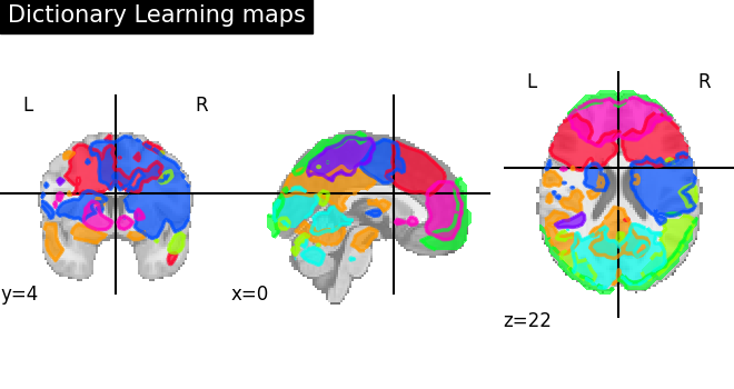
Extract functional networks with Dictionary learning

Import DictLearning from the decomposition module, instantiate the object, and fit the model to the functional datasets

from nilearn.decomposition import DictLearning

# Initialize DictLearning object
dict_learn = DictLearning(
    n_components=8,
    smoothing_fwhm=6.0,
    memory="nilearn_cache",
    memory_level=2,
    random_state=0,
    standardize="zscore_sample",
)
# Fit to the data
dict_learn.fit(func_filenames)
# Resting state networks/maps in attribute `components_img_`
components_img = dict_learn.components_img_

# Visualization of functional networks
# Show networks using plotting utilities
from nilearn import plotting

plotting.plot_prob_atlas(
    components_img,
    view_type="filled_contours",
    title="Dictionary Learning maps",
)

[DictLearning.fit] Resampling mask
/home/remi/github/nilearn/nilearn_doc_build/.tox/doc/lib/python3.9/site-packages/nilearn/plotting/displays/_axes.py:74: UserWarning:

No contour levels were found within the data range.

/home/remi/github/nilearn/nilearn_doc_build/.tox/doc/lib/python3.9/site-packages/nilearn/plotting/displays/_axes.py:74: UserWarning:

linewidths is ignored by contourf


<nilearn.plotting.displays._slicers.OrthoSlicer object at 0x740d17e80ee0>

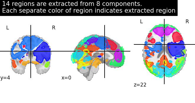
Extract regions from networks

Import RegionExtractor from the regions module. threshold=0.5 indicates that we keep nominal of amount nonzero voxels across all maps, less the threshold means that more intense non-voxels will be survived.

from nilearn.regions import RegionExtractor

extractor = RegionExtractor(
    components_img,
    threshold=0.5,
    thresholding_strategy="ratio_n_voxels",
    extractor="local_regions",
    standardize="zscore_sample",
    standardize_confounds="zscore_sample",
    min_region_size=1350,
)
# Just call fit() to process for regions extraction
extractor.fit()
# Extracted regions are stored in regions_img_
regions_extracted_img = extractor.regions_img_
# Each region index is stored in index_
regions_index = extractor.index_
# Total number of regions extracted
n_regions_extracted = regions_extracted_img.shape[-1]

# Visualization of region extraction results
title = (
    f"{n_regions_extracted} regions are extracted from 8 components.\n"
    "Each separate color of region indicates extracted region"
)
plotting.plot_prob_atlas(
    regions_extracted_img, view_type="filled_contours", title=title
)

/home/remi/github/nilearn/nilearn_doc_build/.tox/doc/lib/python3.9/site-packages/numpy/ma/core.py:2826: UserWarning:

Warning: converting a masked element to nan.

/home/remi/github/nilearn/nilearn_doc_build/.tox/doc/lib/python3.9/site-packages/matplotlib/contour.py:1494: UserWarning:

Warning: converting a masked element to nan.

/home/remi/github/nilearn/nilearn_doc_build/.tox/doc/lib/python3.9/site-packages/matplotlib/contour.py:1495: UserWarning:

Warning: converting a masked element to nan.


<nilearn.plotting.displays._slicers.OrthoSlicer object at 0x740cfb0ec220>

Compute correlation coefficients

First we need to do subjects timeseries signals extraction and then estimating correlation matrices on those signals. To extract timeseries signals, we call transform onto each subject functional data stored in func_filenames. To estimate correlation matrices we import connectome utilities from nilearn.

from nilearn.connectome import ConnectivityMeasure

correlations = []
# Initializing ConnectivityMeasure object with kind='correlation'
connectome_measure = ConnectivityMeasure(
    kind="correlation",
    standardize="zscore_sample",
)
for filename, confound in zip(func_filenames, confounds):
    # call transform from RegionExtractor object to extract timeseries signals
    timeseries_each_subject = extractor.transform(filename, confounds=confound)
    # call fit_transform from ConnectivityMeasure object
    correlation = connectome_measure.fit_transform([timeseries_each_subject])
    # saving each subject correlation to correlations
    correlations.append(correlation)

# Mean of all correlations
import numpy as np

mean_correlations = np.mean(correlations, axis=0).reshape(
    n_regions_extracted, n_regions_extracted
)

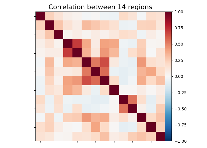
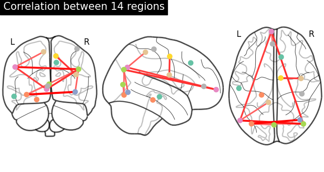
Plot resulting connectomes

First we plot the mean of correlation matrices with plot_matrix, and we use plot_connectome to plot the connectome relations.

title = f"Correlation between {int(n_regions_extracted)} regions"

# First plot the matrix
display = plotting.plot_matrix(
    mean_correlations, vmax=1, vmin=-1, colorbar=True, title=title
)

# Then find the center of the regions and plot a connectome
regions_img = regions_extracted_img
coords_connectome = plotting.find_probabilistic_atlas_cut_coords(regions_img)

plotting.plot_connectome(
    mean_correlations, coords_connectome, edge_threshold="90%", title=title
)

• 
• 

<nilearn.plotting.displays._projectors.OrthoProjector object at 0x740d1fed2b20>

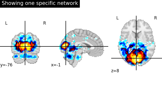
Plot regions extracted for only one specific network

First, we plot a network of index=4 without region extraction (left plot).

from nilearn import image

img = image.index_img(components_img, 4)
coords = plotting.find_xyz_cut_coords(img)
display = plotting.plot_stat_map(
    img,
    cut_coords=coords,
    colorbar=False,
    title="Showing one specific network",
)

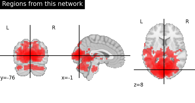
Now, we plot (right side) same network after region extraction to show that connected regions are nicely separated. Each brain extracted region is identified as separate color.

For this, we take the indices of the all regions extracted related to original network given as 4.

regions_indices_of_map3 = np.where(np.array(regions_index) == 4)

display = plotting.plot_anat(
    cut_coords=coords, title="Regions from this network"
)

# Add as an overlay all the regions of index 4
colors = "rgbcmyk"
for each_index_of_map3, color in zip(regions_indices_of_map3[0], colors):
    display.add_overlay(
        image.index_img(regions_extracted_img, each_index_of_map3),
        cmap=plotting.cm.alpha_cmap(color),
    )

plotting.show()

/home/remi/github/nilearn/nilearn_doc_build/.tox/doc/lib/python3.9/site-packages/numpy/ma/core.py:2826: UserWarning:

Warning: converting a masked element to nan.

Estimated memory usage: 1494 MB