Note
This page is a reference documentation. It only explains the function signature, and not how to use it. Please refer to the user guide for the big picture.
nilearn.plotting.plot_prob_atlas
- nilearn.plotting.plot_prob_atlas(maps_img, bg_img=<MNI152Template>, view_type='auto', threshold='auto', linewidths=2.5, cut_coords=None, output_file=None, display_mode='ortho', figure=None, axes=None, title=None, annotate=True, draw_cross=True, black_bg='auto', dim='auto', colorbar=True, cmap='gist_rainbow', vmin=None, vmax=None, alpha=0.7, radiological=False, **kwargs)[source]
Plot a Probabilistic atlas onto the anatomical image by default MNI template.
- Parameters:
- maps_imgNiimg-like object or the filename
4D image of the Probabilistic atlas maps.
- bg_imgNiimg-like object, optional
See Input and output: neuroimaging data representation. The background image to plot on top of. If nothing is specified, the MNI152 template will be used. To turn off background image, just pass “bg_img=False”. default=MNI152TEMPLATE.
Added in Nilearn 0.4.0.
- view_type{‘auto’, ‘contours’, ‘filled_contours’, ‘continuous’}, default=’auto’
If view_type == ‘auto’, it means maps will be displayed automatically using any one of the three view types. The automatic selection of view type depends on the total number of maps. If view_type == ‘contours’, maps are overlaid as contours If view_type == ‘filled_contours’, maps are overlaid as contours along with color fillings inside the contours. If view_type == ‘continuous’, maps are overlaid as continuous colors irrespective of the number maps.
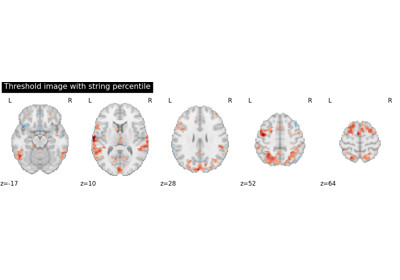
- thresholda
intorfloatorstrorlistofintorfloatorstr, default=’auto’ This parameter is optional and is used to threshold the maps image using the given value or automatically selected value. The values in the image (in absolute value) above the threshold level will be visualized. The default strategy, computes a threshold level that seeks to minimize (yet not eliminate completely) the overlap between several maps for a better visualization. The threshold can also be expressed as a percentile over the values of the whole atlas. In that case, the value must be specified as string finishing with a percent sign, e.g., “25.3%”. If a single string is provided, the same percentile will be applied over the whole atlas. Otherwise, if a list of percentiles is provided, each 3D map is thresholded with certain percentile sequentially. Length of percentiles given should match the number of 3D map in time (4th) dimension. If a number or a list of numbers, the numbers should be non-negative. The given value will be used directly to threshold the maps without any percentile calculation. If None, a very small threshold is applied to remove numerical noise from the maps background.
- linewidths
float, optional Set the boundary thickness of the contours. Only reflects when view_type=contours. default=2.5.
- cut_coordsNone, allowed types depend on the
display_mode, optional The world coordinates of the point where the cut is performed.
If
display_modeis'ortho'or'tiled', this must be a 3-sequence offloatorint:(x, y, z).If
display_modeis'xz','yz'or'yx', this must be a 2-sequence offloatorint:(x, z),(y, z)or(x, y).If
display_modeis"x","y", or"z", this can be:If
display_modeis'mosaic', this can be:an
intin which case it specifies the number of cuts to perform in each direction"x","y","z".a 3-sequence of
floatorintin which case it specifies the number of cuts to perform in each direction"x","y","z"separately.dict<str: 1Dndarray> in which case keys are the directions (‘x’, ‘y’, ‘z’) and the values are sequences holding the cut coordinates.
If
Noneis given, the cuts are calculated automatically.
- output_file
strorpathlib.Pathor None, default=None The name of an image file to export the plot to. Valid extensions are .png, .pdf, .svg. If output_file is not None, the plot is saved to a file, and the display is closed.
- display_mode{“ortho”, “tiled”, “mosaic”, “x”, “y”, “z”, “yx”, “xz”, “yz”}, default=”ortho”
Choose the direction of the cuts:
"x": sagittal"y": coronal"z": axial"ortho": three cuts are performed in orthogonal directions"tiled": three cuts are performed and arranged in a 2x2 grid"mosaic": three cuts are performed along multiple rows and columns
- figure
int, ormatplotlib.figure.Figure, or None, optional Matplotlib figure used or its number. If None is given, a new figure is created.
- axes
matplotlib.axes.Axes, or 4tupleoffloat: (xmin, ymin, width, height), default=None The axes, or the coordinates, in matplotlib figure space, of the axes used to display the plot. If None, the complete figure is used.
- title
str, or None, default=None The title displayed on the figure.
- annotate
bool, default=True If annotate is True (like positions and / or left/right annotation) are added to the plot.
- draw_cross
bool, default=True If draw_cross is True, a cross is drawn on the plot to indicate the cut position.
- black_bg
bool, or “auto”, optional If True, the background of the image is set to be black. If you wish to save figures with a black background, you will need to pass facecolor=”k”, edgecolor=”k” to
matplotlib.pyplot.savefig. default=’auto’.- dim
float, or “auto”, optional Dimming factor applied to background image. By default, automatic heuristics are applied based upon the background image intensity. Accepted float values, where a typical span is between -2 and 2 (-2 = increase contrast; 2 = decrease contrast), but larger values can be used for a more pronounced effect. 0 means no dimming. default=’auto’.
- cmap
matplotlib.colors.Colormap, orstr, optional The colormap to use. Either a string which is a name of a matplotlib colormap, or a matplotlib colormap object. default=`gist_rainbow`.
- colorbar
bool, optional If True, display a colorbar next to the plots. default=True.
- vmin
floator obj:int or None, optional Lower bound of the colormap. The values below vmin are masked. If None, the min of the image is used. Passed to
matplotlib.pyplot.imshow.- vmax
floator obj:int or None, optional Upper bound of the colormap. The values above vmax are masked. If None, the max of the image is used. Passed to
matplotlib.pyplot.imshow.- alpha
floatbetween 0 and 1, default=0.7 Alpha sets the transparency of the color inside the filled contours.
- radiological
bool, default=False Invert x axis and R L labels to plot sections as a radiological view. If False (default), the left hemisphere is on the left of a coronal image. If True, left hemisphere is on the right.
- kwargsextra keyword arguments, optional
Extra keyword arguments ultimately passed to matplotlib.pyplot.imshow via
add_overlay.
- Returns:
- display
OrthoSliceror None An instance of the OrthoSlicer class. If
output_fileis defined, None is returned.
- display
- Raises:
- ValueError
if the specified threshold is a negative number
See also
nilearn.plotting.plot_roiTo simply plot max-prob atlases (3D images)
Examples using nilearn.plotting.plot_prob_atlas
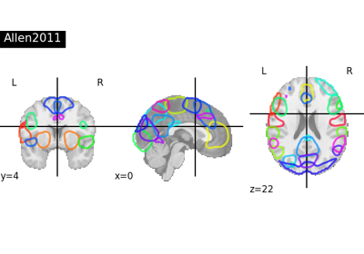
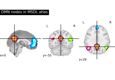
Visualizing a probabilistic atlas: the default mode in the MSDL atlas
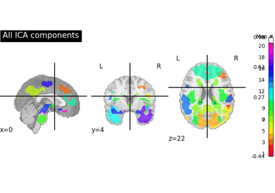
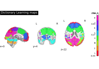
Deriving spatial maps from group fMRI data using ICA and Dictionary Learning
Regions extraction using dictionary learning and functional connectomes
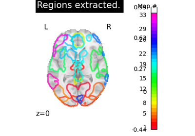
Regions Extraction of Default Mode Networks using Smith Atlas