Making a surface plot of a 3D statistical map

In this example, we will project a 3D statistical map onto a cortical mesh using SurfaceImage, display a surface plot of the projected map using plot_surf_stat_map with different plotting engines, and add contours of regions of interest using plot_surf_contours.

Sample the 3D data around each node of the mesh

You can create a SurfaceImage object from a nifti image by using the from_volume class method. that will call indirectly vol_to_surf.

Get a statistical map as nifti

from nilearn.datasets import load_sample_motor_activation_image

stat_img = load_sample_motor_activation_image()

Get a cortical mesh

from nilearn.datasets import load_fsaverage

fsaverage_meshes = load_fsaverage()

Construct a surface image from a volume.

from nilearn.surface import SurfaceImage

surface_image = SurfaceImage.from_volume(
    mesh=fsaverage_meshes["pial"],
    volume_img=stat_img,
)

Here, we load the curvature map to use as background map some plots. We define a surface map whose value for a given vertex is 1 if the curvature is positive, -1 if the curvature is negative.

import numpy as np

from nilearn.datasets import load_fsaverage_data

curv_sign = load_fsaverage_data(data_type="curvature")
for hemi, data in curv_sign.data.parts.items():
    curv_sign.data.parts[hemi] = np.sign(data)

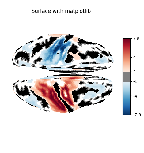
Plot the surface image

You can visualize the surface image using the function plot_surf_stat_map which uses matplotlib as the default plotting engine.

from nilearn.plotting import plot_surf_stat_map

# In this example we will only plot the right hemisphere
hemi = "right"

fig = plot_surf_stat_map(
    stat_map=surface_image,
    surf_mesh=fsaverage_meshes["inflated"],
    hemi=hemi,
    title="Surface with matplotlib",
    colorbar=True,
    threshold=1.0,
    bg_map=curv_sign,
)
fig.show()

Interactive plotting with Plotly

If you have a recent version of Nilearn (>=0.8.2), and if you have plotly installed, you can easily configure plot_surf_stat_map to use plotly instead of matplotlib:

engine = "plotly"
# If plotly is not installed, use matplotlib
from nilearn._utils.helpers import is_plotly_installed

if not is_plotly_installed():
    engine = "matplotlib"

print(f"Using plotting engine {engine}.")

figure = plot_surf_stat_map(
    stat_map=surface_image,
    surf_mesh=fsaverage_meshes["inflated"],
    hemi=hemi,
    title=f"Surface with {engine}",
    colorbar=True,
    threshold=1.0,
    bg_map=curv_sign,
    bg_on_data=True,
    engine=engine,  # Specify the plotting engine here
)

# Uncomment the line below
# to view the figure in browser.
# figure.show()

Using plotting engine plotly.
/home/remi/github/nilearn/nilearn_doc_build/.tox/doc/lib/python3.9/site-packages/nilearn/plotting/surf_plotting.py:1017: UserWarning: vmin cannot be chosen when cmap is symmetric
  fig = _plot_surf_plotly(

When using matplolib as the plotting engine, a standard matplotlib.figure.Figure is returned. With plotly as the plotting engine, a custom PlotlySurfaceFigure is returned which provides a similar API to the Figure. For example, you can save a static version of the figure to file (this option requires to have kaleido installed):

# Save the figure as we would do with a matplotlib figure.
# Uncomment the following line to save the previous figure to file
# fig.savefig("right_hemisphere.png")

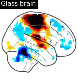
Plot 3D image for comparison

from nilearn.plotting import plot_glass_brain, plot_stat_map, show

plot_glass_brain(
    stat_map_img=stat_img,
    display_mode="r",
    plot_abs=False,
    title="Glass brain",
    threshold=2.0,
)

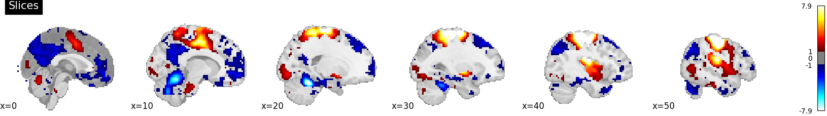
plot_stat_map(
    stat_map_img=stat_img,
    display_mode="x",
    threshold=1.0,
    cut_coords=range(0, 51, 10),
    title="Slices",
)

• 
• 

<nilearn.plotting.displays._slicers.XSlicer object at 0x740d1a8d0e20>

Use an atlas and choose regions to outline

from nilearn.datasets import fetch_atlas_surf_destrieux

fsaverage = load_fsaverage("fsaverage5")
destrieux = fetch_atlas_surf_destrieux()
destrieux_atlas = SurfaceImage(
    mesh=fsaverage["inflated"],
    data={
        "left": destrieux["map_left"],
        "right": destrieux["map_right"],
    },
)

# The labels are stored as bytes for the Destrieux atlas.
# For convenience we decode them to string.
label_names = [x.decode("utf-8") for x in destrieux.labels]

# these are the regions we want to outline
regions_dict = {
    "G_postcentral": "Postcentral gyrus",
    "G_precentral": "Precentral gyrus",
}

# get indices in atlas for these labels
regions_indices = [
    np.where(np.array(label_names) == region)[0][0] for region in regions_dict
]

labels = list(regions_dict.values())

[get_dataset_dir] Dataset found in /home/remi/nilearn_data/destrieux_surface

Display outlines of the regions of interest on top of a statistical map

from nilearn.plotting import plot_surf_contours

fsaverage_sulcal = load_fsaverage_data(data_type="sulcal", mesh_type="pial")

figure = plot_surf_stat_map(
    stat_map=surface_image,
    surf_mesh=fsaverage_meshes["inflated"],
    hemi=hemi,
    title="ROI outlines on surface",
    colorbar=True,
    threshold=1.0,
    bg_map=fsaverage_sulcal,
    engine=engine,
)
if engine == "matplotlib":
    plot_surf_contours(
        roi_map=destrieux_atlas,
        hemi=hemi,
        labels=labels,
        levels=regions_indices,
        figure=figure,
        legend=True,
        colors=["g", "k"],
    )
    show()
elif engine == "plotly":
    figure.add_contours(
        roi_map=destrieux_atlas,
        levels=regions_indices,
        labels=labels,
        lines=[{"width": 5}],
        hemi=hemi,
    )
    # view the contours in a browser
    # figure.show()

/home/remi/github/nilearn/nilearn_doc_build/.tox/doc/lib/python3.9/site-packages/nilearn/plotting/surf_plotting.py:1017: UserWarning:

vmin cannot be chosen when cmap is symmetric

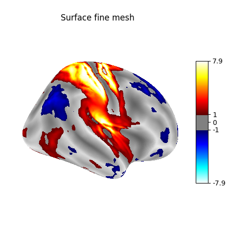
Plot with higher-resolution mesh

load_fsaverage and load_fsaverage_data take a mesh argument which specifies whether to fetch the low-resolution fsaverage5 mesh, or another mesh like the high-resolution fsaverage mesh. Using mesh="fsaverage" will result in more memory usage and computation time, but finer visualizations.

big_fsaverage_meshes = load_fsaverage(mesh="fsaverage")

big_fsaverage_sulcal = load_fsaverage_data(
    mesh="fsaverage",
    data_type="sulcal",
    mesh_type="inflated",
)

big_img = SurfaceImage.from_volume(
    mesh=big_fsaverage_meshes["pial"],
    volume_img=stat_img,
)

plot_surf_stat_map(
    stat_map=big_img,
    surf_mesh=big_fsaverage_meshes["inflated"],
    hemi=hemi,
    colorbar=True,
    title="Surface fine mesh",
    threshold=1.0,
    bg_map=big_fsaverage_sulcal,
)
show()

[get_dataset_dir] Dataset found in /home/remi/nilearn_data/fsaverage
[get_dataset_dir] Dataset found in /home/remi/nilearn_data/fsaverage
[get_dataset_dir] Dataset found in /home/remi/nilearn_data/fsaverage

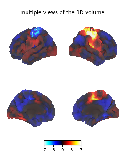
Plot multiple views of the 3D volume on a surface

plot_img_on_surf takes a nifti statistical map and projects it onto a surface. It supports multiple choices of orientations, and can plot either one or both hemispheres. If no surf_mesh is given, plot_img_on_surf projects the images onto FreeSurfer's fsaverage5.

from nilearn.plotting import plot_img_on_surf

plot_img_on_surf(
    stat_map=stat_img,
    views=["lateral", "medial"],
    hemispheres=["left", "right"],
    colorbar=True,
    title="multiple views of the 3D volume",
    bg_on_data=True,
)
show()

3D visualization in a web browser

An alternative to plot_surf_stat_map is to use view_surf or view_img_on_surf that give more interactive visualizations in a web browser. See 3D Plots of statistical maps or atlases on the cortical surface for more details.

from nilearn.plotting import view_surf

view = view_surf(
    surf_mesh=fsaverage_meshes["inflated"],
    surf_map=surface_image,
    threshold="90%",
    bg_map=fsaverage_sulcal,
    hemi="right",
    title="3D visualization in a web browser",
)

# In a Jupyter notebook, if ``view`` is the output of a cell,
# it will be displayed below the cell
view
# view.open_in_browser()

# We don't need to do the projection ourselves, we can use
# :func:`~nilearn.plotting.view_img_on_surf`:
from nilearn.plotting import view_img_on_surf

view = view_img_on_surf(stat_img, threshold="90%")

view
# view.open_in_browser()

Impact of plot parameters on visualization

You can specify arguments to be passed on to the function vol_to_surf using vol_to_surf_kwargs This allows fine-grained control of how the input 3D image is resampled and interpolated - for example if you are viewing a volumetric atlas, you would want to avoid averaging the labels between neighboring regions. Using nearest-neighbor interpolation with zero radius will achieve this.

from nilearn.datasets import fetch_atlas_destrieux_2009

destrieux = fetch_atlas_destrieux_2009(legacy_format=False)

view = view_img_on_surf(
    stat_map_img=destrieux.maps,
    surf_mesh="fsaverage",
    cmap="tab20",
    vol_to_surf_kwargs={
        "n_samples": 1,
        "radius": 0.0,
        "interpolation": "nearest",
    },
    symmetric_cmap=False,
    colorbar=False,
)

view
# view.open_in_browser()

[get_dataset_dir] Dataset found in /home/remi/nilearn_data/destrieux_2009
[get_dataset_dir] Dataset found in /home/remi/nilearn_data/fsaverage

Estimated memory usage: 680 MB