Note

This page is a reference documentation. It only explains the function signature, and not how to use it. Please refer to the user guide for the big picture.

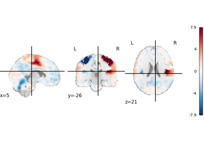
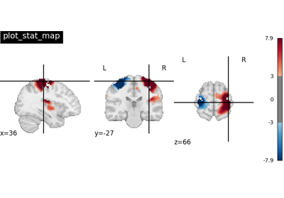
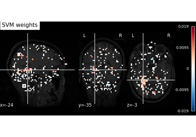
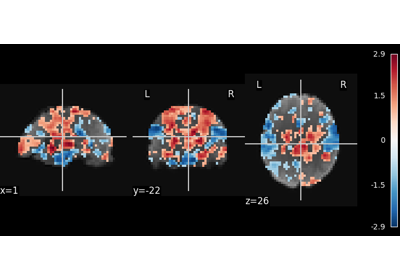
nilearn.plotting.plot_stat_map¶

nilearn.plotting.plot_stat_map(stat_map_img, bg_img=<MNI152Template>, cut_coords=None, output_file=None, display_mode='ortho', colorbar=True, cbar_tick_format='%.2g', figure=None, axes=None, title=None, threshold=1e-06, annotate=True, draw_cross=True, black_bg='auto', cmap='RdBu_r', symmetric_cbar='auto', dim='auto', vmin=None, vmax=None, radiological=False, resampling_interpolation='continuous', transparency=None, transparency_range=None, **kwargs)[source]¶

Plot cuts of an ROI/mask image.

By default 3 cuts: Frontal, Axial, and Lateral.

Parameters:

stat_map_imgNiimg-like object

See Input and output: neuroimaging data representation. The statistical map image

bg_imgNiimg-like object, optional

See Input and output: neuroimaging data representation. The background image to plot on top of. If nothing is specified, the MNI152 template will be used. To turn off background image, just pass “bg_img=None”. Default=MNI152TEMPLATE.

cut_coordsNone, a tuple of float, or int, optional

The MNI coordinates of the point where the cut is performed.

If display_mode is ‘ortho’ or ‘tiled’, this should be a 3-tuple: (x, y, z)
For display_mode == “x”, “y”, or “z”, then these are the coordinates of each cut in the corresponding direction.
If None is given, the cuts are calculated automatically.
If display_mode is ‘mosaic’, and the number of cuts is the same for all directions, cut_coords can be specified as an integer. It can also be a length 3 tuple specifying the number of cuts for every direction if these are different.

Note

If display_mode is “x”, “y” or “z”, cut_coords can be an integer, in which case it specifies the number of cuts to perform.

output_filestr or pathlib.Path or None, optional

The name of an image file to export the plot to. Valid extensions are .png, .pdf, .svg. If output_file is not None, the plot is saved to a file, and the display is closed.

display_mode{“ortho”, “tiled”, “mosaic”, “x”, “y”, “z”, “yx”, “xz”, “yz”}, default=”ortho”

Choose the direction of the cuts:

"x": sagittal
"y": coronal
"z": axial
"ortho": three cuts are performed in orthogonal directions
"tiled": three cuts are performed and arranged in a 2x2 grid
"mosaic": three cuts are performed along multiple rows and columns

colorbarbool, optional

If True, display a colorbar on the right of the plots. Default=True.

cbar_tick_formatstr, default=”%.2g” (scientific notation)

Controls how to format the tick labels of the colorbar. Ex: use “%i” to display as integers.

figureint, or matplotlib.figure.Figure, or None, optional

Matplotlib figure used or its number. If None is given, a new figure is created.

axesmatplotlib.axes.Axes, or 4 tuple of float: (xmin, ymin, width, height), default=None

The axes, or the coordinates, in matplotlib figure space, of the axes used to display the plot. If None, the complete figure is used.

titlestr, or None, default=None

The title displayed on the figure.

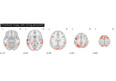
thresholdint or float, None, or ‘auto’, optional

If None is given, the image is not thresholded. If number is given, it must be non-negative. The specified value is used to threshold the image: values below the threshold (in absolute value) are plotted as transparent. If “auto” is given, the threshold is determined based on the score obtained using percentile value “80%” on the absolute value of the image data. Default=1e-6.

annotatebool, default=True

If annotate is True, positions and left/right annotation are added to the plot.

draw_crossbool, default=True

If draw_cross is True, a cross is drawn on the plot to indicate the cut position.

black_bgbool, or “auto”, optional

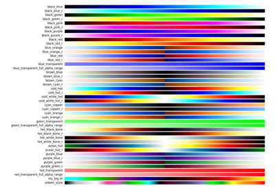
If True, the background of the image is set to be black. If you wish to save figures with a black background, you will need to pass facecolor=”k”, edgecolor=”k” to matplotlib.pyplot.savefig. Default=’auto’.

cmapmatplotlib.colors.Colormap, or str, optional

The colormap to use. Either a string which is a name of a matplotlib colormap, or a matplotlib colormap object.

Default=default=”RdBu_r”.

symmetric_cbarbool, or “auto”, default=”auto”

Specifies whether the colorbar and colormap should range from -vmax to vmax (or from vmin to -vmin if -vmin is greater than vmax) or from vmin to vmax. Setting to “auto” (the default) will select the former if either vmin or vmax is None and the image has both positive and negative values.

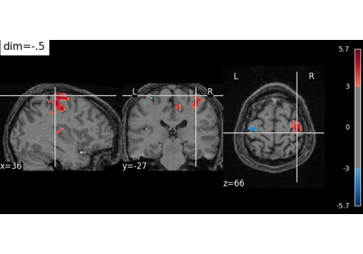
dimfloat, or “auto”, optional

Dimming factor applied to background image. By default, automatic heuristics are applied based upon the background image intensity. Accepted float values, where a typical span is between -2 and 2 (-2 = increase contrast; 2 = decrease contrast), but larger values can be used for a more pronounced effect. 0 means no dimming. Default=’auto’.

vminfloat or obj:int or None, optional

Lower bound of the colormap. The values below vmin are masked. If None, the min of the image is used. Passed to matplotlib.pyplot.imshow.

vmaxfloat or obj:int or None, optional

Upper bound of the colormap. The values above vmax are masked. If None, the max of the image is used. Passed to matplotlib.pyplot.imshow.

resampling_interpolationstr, optional

Interpolation to use when resampling the image to the destination space. Can be:

"continuous": use 3rd-order spline interpolation
"nearest": use nearest-neighbor mapping.

Note

"nearest" is faster but can be noisier in some cases.

Default=’continuous’.

radiologicalbool, default=False

Invert x axis and R L labels to plot sections as a radiological view. If False (default), the left hemisphere is on the left of a coronal image. If True, left hemisphere is on the right.

transparencyfloat between 0 and 1, or a Niimg-Like object, or None, default = None

Value to be passed as alpha value to imshow. if None is passed, it will be set to 1. If an image is passed, voxel-wise alpha blending will be applied, by relying on the absolute value of transparency at each voxel.

Added in version 0.12.0.

transparency_rangetuple or list of 2 non-negative numbers, or None, default = None

When an image is passed to transparency, this determines the range of values in the image to use for transparency (alpha blending). For example with transparency_range = [1.96, 3], any voxel / vertex ( $v_i$ ):

with a value between between -1.96 and 1.96, would be fully transparent (alpha = 0),
with a value less than -3 or greater than 3, would be fully opaque (alpha = 1),
with a value in the intervals [-3.0, -1.96] or [1.96, 3.0], would have an alpha_i value scaled linearly between 0 and 1 : $alpha_i = (\lvert v_i \lvert - 1.96) / (3.0 - 1.96)$ .

This parameter will be ignored unless an image is passed as transparency. The first number must be greater than 0 and less than the second one. if None is passed, this will be set to [0, max(abs(transparency))].

Added in version 0.12.0.

kwargsextra keyword arguments, optional

Extra keyword arguments ultimately passed to matplotlib.pyplot.imshow via add_overlay.

Returns:

displayOrthoSlicer or None: An instance of the OrthoSlicer class. If output_file is defined, None is returned.

Raises:

ValueError: if the specified threshold is a negative number

Examples using `nilearn.plotting.plot_stat_map`¶

3D and 4D niimgs: handling and visualizing

Intro to GLM Analysis: a single-run, single-subject fMRI dataset

Colormaps in Nilearn

Controlling the contrast of the background when plotting

Making a surface plot of a 3D statistical map

More plotting tools from nilearn

Plotting images with transparent thresholding

Plotting tools in nilearn

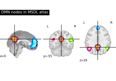
Visualizing a probabilistic atlas: the default mode in the MSDL atlas

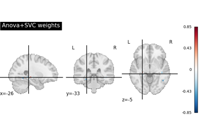
Decoding with ANOVA + SVM: face vs house in the Haxby dataset

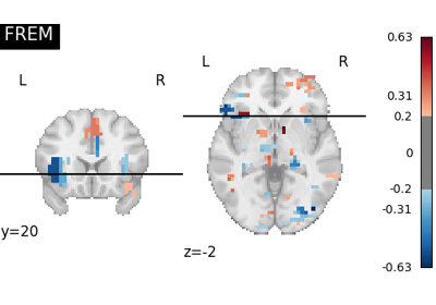
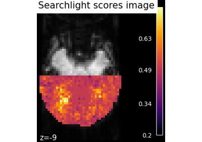
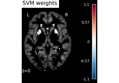
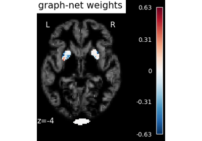
Decoding with FREM: face vs house vs chair object recognition

Different classifiers in decoding the Haxby dataset

Encoding models for visual stimuli from Miyawaki et al. 2008

FREM on Jimura et al “mixed gambles” dataset

FREM on Jimura et al "mixed gambles" dataset

Searchlight analysis of face vs house recognition

Voxel-Based Morphometry on Oasis dataset

Voxel-Based Morphometry on Oasis dataset with Space-Net prior

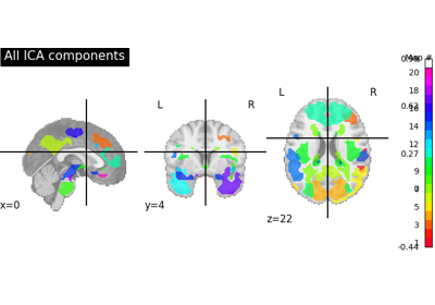
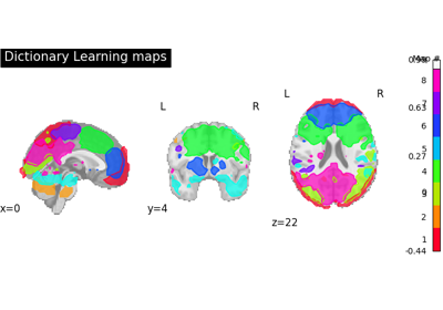
Deriving spatial maps from group fMRI data using ICA and Dictionary Learning

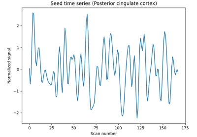
Producing single subject maps of seed-to-voxel correlation

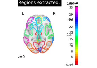
Regions extraction using dictionary learning and functional connectomes

Analysis of an fMRI dataset with a Finite Impule Response (FIR) model

Default Mode Network extraction of ADHD dataset

Predicted time series and residuals

Simple example of two-runs fMRI model fitting

Single-subject data (two runs) in native space

Understanding parameters of the first-level model

Example of generic design in second-level models

Second-level fMRI model: true positive proportion in clusters

Statistical testing of a second-level analysis

Voxel-Based Morphometry on OASIS dataset

Comparing the means of 2 images

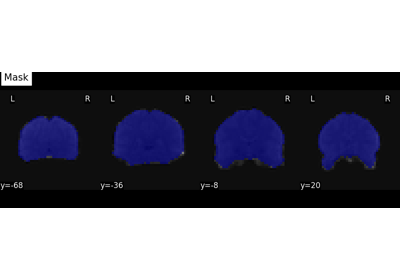
Computing a Region of Interest (ROI) mask manually

Image thresholding

Negating an image with math_img

Region Extraction using a t-statistical map (3D)

Regions Extraction of Default Mode Networks using Smith Atlas

Resample an image to a template

Simple example of NiftiMasker use

Advanced decoding using scikit learn

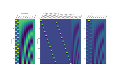
Beta-Series Modeling for Task-Based Functional Connectivity and Decoding

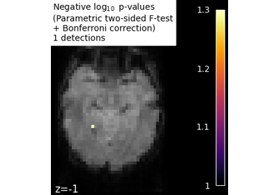
Massively univariate analysis of a calculation task from the Localizer dataset

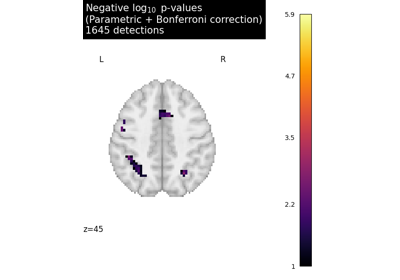
Massively univariate analysis of face vs house recognition

Multivariate decompositions: Independent component analysis of fMRI

NeuroVault cross-study ICA maps

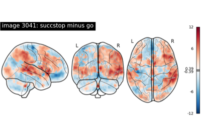
NeuroVault meta-analysis of stop-go paradigm studies

nilearn.plotting.plot_stat_map¶

Examples using nilearn.plotting.plot_stat_map¶

Examples using `nilearn.plotting.plot_stat_map`¶