Note

This page is a reference documentation. It only explains the function signature, and not how to use it. Please refer to the user guide for the big picture.

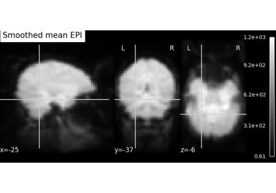
nilearn.plotting.plot_epi¶

nilearn.plotting.plot_epi(epi_img=None, cut_coords=None, output_file=None, display_mode='ortho', figure=None, axes=None, title=None, annotate=True, draw_cross=True, black_bg=True, colorbar=True, cbar_tick_format='%.2g', cmap='gray', vmin=None, vmax=None, radiological=False, **kwargs)[source]¶

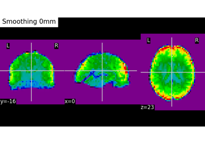
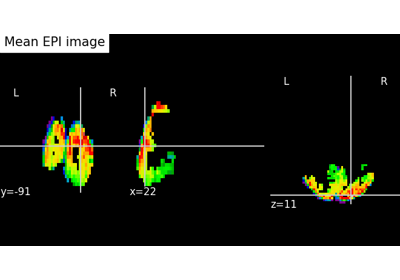
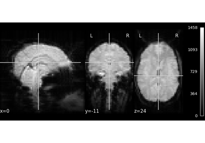
Plot cuts of an EPI image.

By default 3 cuts: Frontal, Axial, and Lateral.

Parameters:

epi_imga Niimg-like object or None, default=None

The EPI (T2*) image.

cut_coordsNone, a tuple of float, or int, optional

The MNI coordinates of the point where the cut is performed.

If display_mode is ‘ortho’ or ‘tiled’, this should be a 3-tuple: (x, y, z)
For display_mode == “x”, “y”, or “z”, then these are the coordinates of each cut in the corresponding direction.
If None is given, the cuts are calculated automatically.
If display_mode is ‘mosaic’, and the number of cuts is the same for all directions, cut_coords can be specified as an integer. It can also be a length 3 tuple specifying the number of cuts for every direction if these are different.

Note

If display_mode is “x”, “y” or “z”, cut_coords can be an integer, in which case it specifies the number of cuts to perform.

output_filestr or pathlib.Path or None, optional

The name of an image file to export the plot to. Valid extensions are .png, .pdf, .svg. If output_file is not None, the plot is saved to a file, and the display is closed.

display_mode{“ortho”, “tiled”, “mosaic”, “x”, “y”, “z”, “yx”, “xz”, “yz”}, default=”ortho”

Choose the direction of the cuts:

"x": sagittal
"y": coronal
"z": axial
"ortho": three cuts are performed in orthogonal directions
"tiled": three cuts are performed and arranged in a 2x2 grid
"mosaic": three cuts are performed along multiple rows and columns

figureint, or matplotlib.figure.Figure, or None, optional

Matplotlib figure used or its number. If None is given, a new figure is created.

axesmatplotlib.axes.Axes, or 4 tuple of float: (xmin, ymin, width, height), default=None

The axes, or the coordinates, in matplotlib figure space, of the axes used to display the plot. If None, the complete figure is used.

titlestr, or None, default=None

The title displayed on the figure.

annotatebool, default=True

If annotate is True, positions and left/right annotation are added to the plot.

draw_crossbool, default=True

If draw_cross is True, a cross is drawn on the plot to indicate the cut position.

black_bgbool, or “auto”, optional

If True, the background of the image is set to be black. If you wish to save figures with a black background, you will need to pass facecolor=”k”, edgecolor=”k” to matplotlib.pyplot.savefig. Default=True.

colorbarbool, optional

If True, display a colorbar on the right of the plots. Default=True

cbar_tick_formatstr, default=”%.2g” (scientific notation)

Controls how to format the tick labels of the colorbar. Ex: use “%i” to display as integers.

cmapmatplotlib.colors.Colormap, or str, optional

The colormap to use. Either a string which is a name of a matplotlib colormap, or a matplotlib colormap object. Default=`gray`.

vminfloat or obj:int or None, optional

Lower bound of the colormap. The values below vmin are masked. If None, the min of the image is used. Passed to matplotlib.pyplot.imshow.

vmaxfloat or obj:int or None, optional

Upper bound of the colormap. The values above vmax are masked. If None, the max of the image is used. Passed to matplotlib.pyplot.imshow.

radiologicalbool, default=False

Invert x axis and R L labels to plot sections as a radiological view. If False (default), the left hemisphere is on the left of a coronal image. If True, left hemisphere is on the right.

kwargsextra keyword arguments, optional

Extra keyword arguments ultimately passed to matplotlib.pyplot.imshow via add_overlay.

Returns:

displayOrthoSlicer or None: An instance of the OrthoSlicer class. If output_file is defined, None is returned.

Notes

Arrays should be passed in numpy convention: (x, y, z) ordered.

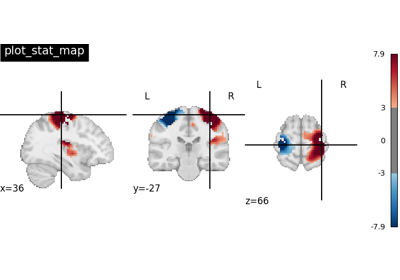
Examples using `nilearn.plotting.plot_epi`¶

A introduction tutorial to fMRI decoding

NeuroImaging volumes visualization

Plotting tools in nilearn

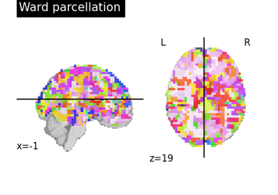
Clustering methods to learn a brain parcellation from fMRI

Computing a Region of Interest (ROI) mask manually

Smoothing an image

Understanding NiftiMasker and mask computation

nilearn.plotting.plot_epi¶

Examples using nilearn.plotting.plot_epi¶

Examples using `nilearn.plotting.plot_epi`¶