Technical point: Illustration of the volume to surface sampling schemes

In nilearn, nilearn.surface.vol_to_surf allows us to measure values of a 3d volume at the nodes of a cortical mesh, transforming it into surface data. This data can then be plotted with nilearn.plotting.plot_surf_stat_map for example.

This script shows, on a toy example, where samples are drawn around each mesh vertex. Image values are interpolated at each sample location, then these samples are averaged to produce a value for the vertex.

Three strategies are available to choose sample locations: they can be spread between corresponding nodes when we have two nested surfaces (e.g. a white matter and a pial surface), along the normal at each node, or inside a ball around each node. Don’t worry too much about choosing one or the other: they take a similar amount of time and give almost identical results for most images. If you do have both pial and white matter surfaces (as for the fsaverage and fsaverage5 surfaces fetched by nilearn.datasets) we recommend passing both to vol_to_surf.

from nilearn._utils.helpers import check_matplotlib

check_matplotlib()

import numpy as np
from matplotlib import pyplot as plt
from matplotlib import tri

from nilearn.surface import surface

Build a mesh (of a cylinder)

N_Z = 5
N_T = 10
u, v = np.mgrid[:N_T, :N_Z]
triangulation = tri.Triangulation(u.flatten(), v.flatten())
angles = u.flatten() * 2 * np.pi / N_T
x, y = np.cos(angles), np.sin(angles)
z = v.flatten() * 2 / N_Z

mesh = [np.asarray([x, y, z]).T, triangulation.triangles]
inner_mesh = [[0.7, 0.7, 1.0] * mesh[0], triangulation.triangles]

Get the locations from which vol_to_surf would draw its samples

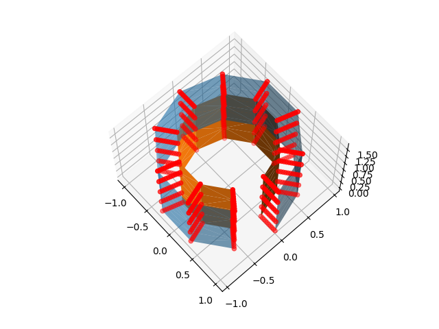
nested_sample_points = surface._sample_locations_between_surfaces(
    mesh, inner_mesh, np.eye(4)
)

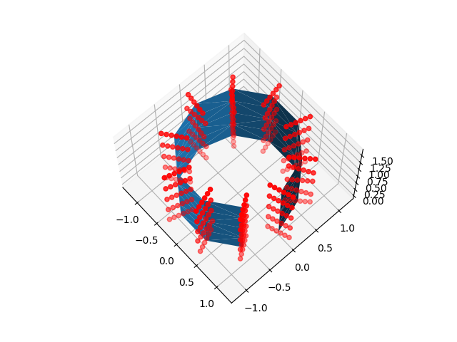
line_sample_points = surface._line_sample_locations(
    mesh, np.eye(4), segment_half_width=0.2, n_points=6
)

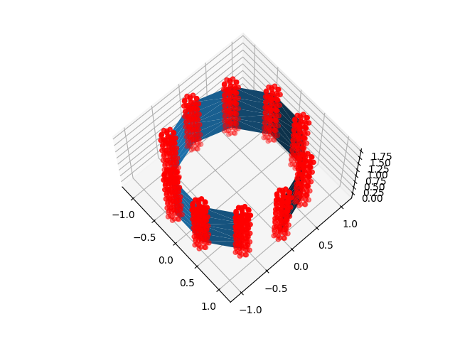
ball_sample_points = surface._ball_sample_locations(
    mesh, np.eye(4), ball_radius=0.15, n_points=20
)

Plot the mesh and the sample locations

fig = plt.figure()
ax = plt.subplot(projection="3d")
ax.view_init(67, -42)
ax.plot_trisurf(x, y, z, triangles=triangulation.triangles, alpha=0.6)
ax.plot_trisurf(*inner_mesh[0].T, triangles=triangulation.triangles)
ax.scatter(*nested_sample_points.T, color="r")

for sample_points in [line_sample_points, ball_sample_points]:
    fig = plt.figure()
    ax = plt.subplot(projection="3d")
    ax.view_init(67, -42)
    ax.plot_trisurf(x, y, z, triangles=triangulation.triangles)
    ax.scatter(*sample_points.T, color="r")

• 
• 
• 

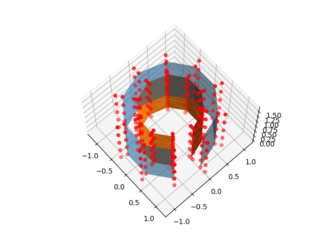
Adjust the sample locations

For “line” and nested surfaces, the depth parameter allows adjusting the position of samples along the line

nested_sample_points = surface._sample_locations_between_surfaces(
    mesh, inner_mesh, np.eye(4), depth=[-0.5, 0.0, 0.8, 1.0, 1.2]
)
fig = plt.figure()
ax = plt.subplot(projection="3d")
ax.view_init(67, -42)
ax.plot_trisurf(x, y, z, triangles=triangulation.triangles, alpha=0.6)
ax.plot_trisurf(*inner_mesh[0].T, triangles=triangulation.triangles)
ax.scatter(*nested_sample_points.T, color="r")

plt.show()

Estimated memory usage: 147 MB