Producing single subject maps of seed-to-voxel correlation

This example shows how to produce seed-to-voxel correlation maps for a single subject based on movie-watching fMRI scans. These maps depict the temporal correlation of a seed region with the rest of the brain.

This example is an advanced one that requires manipulating the data with numpy. Note the difference between images, that lie in brain space, and the numpy array, corresponding to the data inside the mask.

See also for a similar example using cortical surface input data.

Author: Franz Liem

Note

If you are using Nilearn with a version older than 0.9.0, then you should either upgrade your version or import maskers from the input_data module instead of the maskers module.

That is, you should manually replace in the following example all occurrences of:

from nilearn.maskers import NiftiMasker

with:

from nilearn.input_data import NiftiMasker

Getting the data

We will work with the first subject of the brain development fMRI data set. dataset.func is a list of filenames. We select the 1st (0-based) subject by indexing with [0]).

from nilearn import datasets, plotting

dataset = datasets.fetch_development_fmri(n_subjects=1)
func_filename = dataset.func[0]
confound_filename = dataset.confounds[0]

[get_dataset_dir] Dataset found in /home/remi/nilearn_data/development_fmri
[get_dataset_dir] Dataset found in /home/remi/nilearn_data/development_fmri/development_fmri
[get_dataset_dir] Dataset found in /home/remi/nilearn_data/development_fmri/development_fmri

Note that func_filename and confound_filename are strings pointing to files on your hard drive.

print(func_filename)
print(confound_filename)

/home/remi/nilearn_data/development_fmri/development_fmri/sub-pixar123_task-pixar_space-MNI152NLin2009cAsym_desc-preproc_bold.nii.gz
/home/remi/nilearn_data/development_fmri/development_fmri/sub-pixar123_task-pixar_desc-reducedConfounds_regressors.tsv

Time series extraction

We are going to extract signals from the functional time series in two steps. First we will extract the mean signal within the seed region of interest. Second, we will extract the brain-wide voxel-wise time series.

We will be working with one seed sphere in the Posterior Cingulate Cortex (PCC), considered part of the Default Mode Network.

pcc_coords = [(0, -52, 18)]

We use nilearn.maskers.NiftiSpheresMasker to extract the time series from the functional imaging within the sphere. The sphere is centered at pcc_coords and will have the radius we pass the NiftiSpheresMasker function (here 8 mm).

The extraction will also detrend, standardize, and bandpass filter the data. This will create a NiftiSpheresMasker object.

from nilearn.maskers import NiftiSpheresMasker

seed_masker = NiftiSpheresMasker(
    pcc_coords,
    radius=8,
    detrend=True,
    standardize="zscore_sample",
    standardize_confounds="zscore_sample",
    low_pass=0.1,
    high_pass=0.01,
    t_r=2,
    memory="nilearn_cache",
    memory_level=1,
    verbose=0,
)

Then we extract the mean time series within the seed region while regressing out the confounds that can be found in the dataset’s csv file

seed_time_series = seed_masker.fit_transform(
    func_filename, confounds=[confound_filename]
)

Next, we can proceed similarly for the brain-wide voxel-wise time series, using nilearn.maskers.NiftiMasker with the same input arguments as in the seed_masker in addition to smoothing with a 6 mm kernel

from nilearn.maskers import NiftiMasker

brain_masker = NiftiMasker(
    smoothing_fwhm=6,
    detrend=True,
    standardize="zscore_sample",
    standardize_confounds="zscore_sample",
    low_pass=0.1,
    high_pass=0.01,
    t_r=2,
    memory="nilearn_cache",
    memory_level=1,
    verbose=0,
)

Then we extract the brain-wide voxel-wise time series while regressing out the confounds as before

brain_time_series = brain_masker.fit_transform(
    func_filename, confounds=[confound_filename]
)

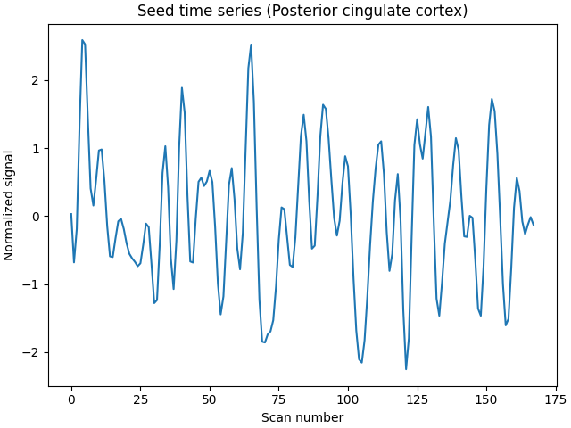
We can now inspect the extracted time series. Note that the seed time series is an array with shape n_volumes, 1), while the brain time series is an array with shape (n_volumes, n_voxels).

print(f"Seed time series shape: ({seed_time_series.shape})")
print(f"Brain time series shape: ({brain_time_series.shape})")

Seed time series shape: ((168, 1))
Brain time series shape: ((168, 32504))

We can plot the seed time series.

import matplotlib.pyplot as plt

plt.figure(constrained_layout=True)

plt.plot(seed_time_series)
plt.title("Seed time series (Posterior cingulate cortex)")
plt.xlabel("Scan number")
plt.ylabel("Normalized signal")

Text(18.166999999999994, 0.5, 'Normalized signal')

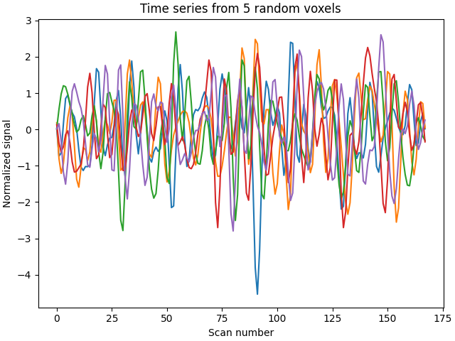
Exemplarily, we can also select 5 random voxels from the brain-wide data and plot the time series from.

plt.figure(constrained_layout=True)

plt.plot(brain_time_series[:, [10, 45, 100, 5000, 10000]])
plt.title("Time series from 5 random voxels")
plt.xlabel("Scan number")
plt.ylabel("Normalized signal")

Text(18.166999999999994, 0.5, 'Normalized signal')

Performing the seed-to-voxel correlation analysis

Now that we have two arrays (sphere signal: (n_volumes, 1), brain-wide voxel-wise signal (n_volumes, n_voxels)), we can correlate the seed signal with the signal of each voxel. The dot product of the two arrays will give us this correlation. Note that the signals have been variance-standardized during extraction. To have them standardized to norm unit, we further have to divide the result by the length of the time series.

import numpy as np

seed_to_voxel_correlations = (
    np.dot(brain_time_series.T, seed_time_series) / seed_time_series.shape[0]
)

The resulting array will contain a value representing the correlation values between the signal in the seed region of interest and each voxel’s signal, and will be of shape (n_voxels, 1). The correlation values can potentially range between -1 and 1.

print(
    "Seed-to-voxel correlation shape: ({}, {})".format(
        *seed_to_voxel_correlations.shape
    )
)
print(
    f"Seed-to-voxel correlation: "
    f"min = {seed_to_voxel_correlations.min():.3f}; "
    f"max = {seed_to_voxel_correlations.max():.3f}"
)

Seed-to-voxel correlation shape: (32504, 1)
Seed-to-voxel correlation: min = -0.642; max = 0.954

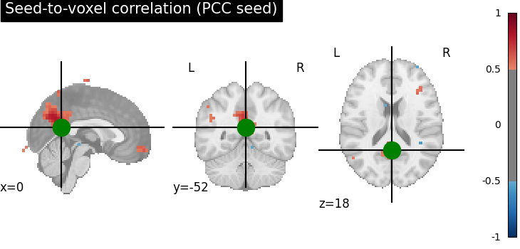
Plotting the seed-to-voxel correlation map

We can now plot the seed-to-voxel correlation map and perform thresholding to only show values more extreme than +/- 0.5. Before displaying, we need to create an in memory Nifti image object. Furthermore, we can display the location of the seed with a sphere and set the cross to the center of the seed region of interest.

seed_to_voxel_correlations_img = brain_masker.inverse_transform(
    seed_to_voxel_correlations.T
)
display = plotting.plot_stat_map(
    seed_to_voxel_correlations_img,
    threshold=0.5,
    vmax=1,
    cut_coords=pcc_coords[0],
    title="Seed-to-voxel correlation (PCC seed)",
)
display.add_markers(
    marker_coords=pcc_coords, marker_color="g", marker_size=300
)
# At last, we save the plot as pdf.
from pathlib import Path

output_dir = Path.cwd() / "results" / "plot_seed_to_voxel_correlation"
output_dir.mkdir(exist_ok=True, parents=True)
print(f"Output will be saved to: {output_dir}")

display.savefig(output_dir / "pcc_seed_correlation.pdf")

Output will be saved to: /home/remi/github/nilearn/nilearn_doc_build/examples/03_connectivity/results/plot_seed_to_voxel_correlation

Fisher-z transformation and save nifti

Finally, we can Fisher-z transform the data to achieve a normal distribution. The transformed array can now have values more extreme than +/- 1.

seed_to_voxel_correlations_fisher_z = np.arctanh(seed_to_voxel_correlations)
print(
    "Seed-to-voxel correlation Fisher-z transformed: "
    f"min = {seed_to_voxel_correlations_fisher_z.min():.3f}; "
    f"max = {seed_to_voxel_correlations_fisher_z.max():.3f}f"
)

Seed-to-voxel correlation Fisher-z transformed: min = -0.762; max = 1.874f

Eventually, we can transform the correlation array back to a Nifti image object, that we can save.

seed_to_voxel_correlations_fisher_z_img = brain_masker.inverse_transform(
    seed_to_voxel_correlations_fisher_z.T
)
seed_to_voxel_correlations_fisher_z_img.to_filename(
    output_dir / "pcc_seed_correlation_z.nii.gz"
)

Estimated memory usage: 1305 MB