Visualizing a probabilistic atlas: the default mode in the MSDL atlas

Visualizing a probabilistic atlas requires visualizing the different maps that compose it.

Here we represent the nodes constituting the default mode network in the MSDL atlas.

The tools that we need to leverage are:

• nilearn.image.index_img to retrieve the various maps composing the atlas

• Adding overlays on an existing brain display, to plot each of these maps

Alternatively, nilearn.plotting.plot_prob_atlas allows to plot the maps in one step that with less control over the plot (see below)

Fetching Probabilistic atlas - MSDL atlas

from nilearn import datasets

atlas_data = datasets.fetch_atlas_msdl()
atlas_filename = atlas_data.maps

[get_dataset_dir] Dataset found in /home/remi/nilearn_data/msdl_atlas

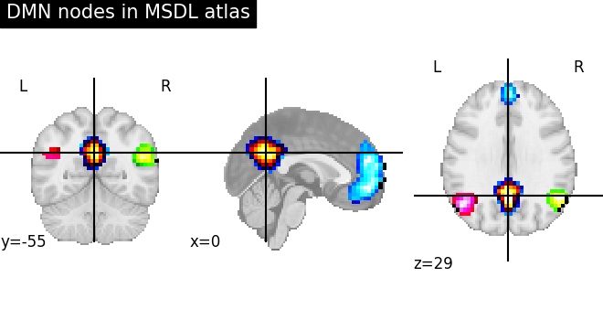
Visualizing a probabilistic atlas with plot_stat_map and add_overlay object

from nilearn import image, plotting

# First plot the map for the PCC: index 4 in the atlas
display = plotting.plot_stat_map(
    image.index_img(atlas_filename, 4),
    colorbar=False,
    title="DMN nodes in MSDL atlas",
)

# Now add as an overlay the maps for the ACC and the left and right
# parietal nodes
cmaps = [
    plotting.cm.black_blue,
    plotting.cm.black_green,
    plotting.cm.black_pink,
]
for index, cmap in zip([5, 6, 3], cmaps):
    display.add_overlay(image.index_img(atlas_filename, index), cmap=cmap)

plotting.show()

/home/remi/github/nilearn/nilearn_doc_build/.tox/doc/lib/python3.9/site-packages/numpy/ma/core.py:2826: UserWarning: Warning: converting a masked element to nan.
  _data = np.array(data, dtype=dtype, copy=copy,

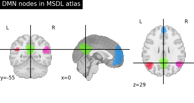
Visualizing a probabilistic atlas with plot_prob_atlas

Alternatively, we can create a new 4D-image by selecting the 3rd, 4th, 5th and 6th (zero-based) probabilistic map from atlas via nilearn.image.index_img and use nilearn.plotting.plot_prob_atlas (added in version 0.2) to plot the selected nodes in one step.

Unlike nilearn.plotting.plot_stat_map this works with 4D images

dmn_nodes = image.index_img(atlas_filename, [3, 4, 5, 6])
# Note that dmn_node is now a 4D image
print(dmn_nodes.shape)

(40, 48, 35, 4)

display = plotting.plot_prob_atlas(
    dmn_nodes, cut_coords=(0, -55, 29), title="DMN nodes in MSDL atlas"
)
plotting.show()

Estimated memory usage: 148 MB