Functional connectivity predicts age group

This example compares different kinds of functional connectivity between regions of interest : correlation, partial correlation, and tangent space embedding.

The resulting connectivity coefficients can be used to discriminate children from adults. In general, the tangent space embedding outperforms the standard correlations: see Dadi et al.[1] for a careful study.

Note

If you are using Nilearn with a version older than 0.9.0, then you should either upgrade your version or import maskers from the input_data module instead of the maskers module.

That is, you should manually replace in the following example all occurrences of:

from nilearn.maskers import NiftiMasker

with:

from nilearn.input_data import NiftiMasker

try:
    import matplotlib.pyplot as plt
except ImportError:
    raise RuntimeError("This script needs the matplotlib library")

Load brain development fMRI dataset and MSDL atlas

We study only 60 subjects from the dataset, to save computation time.

from nilearn import datasets

development_dataset = datasets.fetch_development_fmri(n_subjects=60)

We use probabilistic regions of interest (ROIs) from the MSDL atlas.

from nilearn.maskers import NiftiMapsMasker

msdl_data = datasets.fetch_atlas_msdl()
msdl_coords = msdl_data.region_coords

masker = NiftiMapsMasker(
    msdl_data.maps,
    resampling_target="data",
    t_r=2,
    detrend=True,
    low_pass=0.1,
    high_pass=0.01,
    memory="nilearn_cache",
    memory_level=1,
    standardize="zscore_sample",
    standardize_confounds="zscore_sample",
).fit()

masked_data = [
    masker.transform(func, confounds)
    for (func, confounds) in zip(
        development_dataset.func, development_dataset.confounds
    )
]

What kind of connectivity is most powerful for classification?

we will use connectivity matrices as features to distinguish children from adults. We use cross-validation and measure classification accuracy to compare the different kinds of connectivity matrices.

# prepare the classification pipeline
from sklearn.dummy import DummyClassifier
from sklearn.model_selection import GridSearchCV
from sklearn.pipeline import Pipeline
from sklearn.svm import LinearSVC

from nilearn.connectome import ConnectivityMeasure

kinds = ["correlation", "partial correlation", "tangent"]

pipe = Pipeline(
    [
        (
            "connectivity",
            ConnectivityMeasure(
                vectorize=True,
                standardize="zscore_sample",
            ),
        ),
        (
            "classifier",
            GridSearchCV(LinearSVC(dual=True), {"C": [0.1, 1.0, 10.0]}, cv=5),
        ),
    ]
)

param_grid = [
    {"classifier": [DummyClassifier(strategy="most_frequent")]},
    {"connectivity__kind": kinds},
]

We use random splits of the subjects into training/testing sets. StratifiedShuffleSplit allows preserving the proportion of children in the test set.

from sklearn.model_selection import GridSearchCV, StratifiedShuffleSplit
from sklearn.preprocessing import LabelEncoder

groups = [pheno["Child_Adult"] for pheno in development_dataset.phenotypic]
classes = LabelEncoder().fit_transform(groups)

cv = StratifiedShuffleSplit(n_splits=30, random_state=0, test_size=10)
gs = GridSearchCV(
    pipe,
    param_grid,
    scoring="accuracy",
    cv=cv,
    verbose=1,
    refit=False,
    n_jobs=2,
)
gs.fit(masked_data, classes)
mean_scores = gs.cv_results_["mean_test_score"]
scores_std = gs.cv_results_["std_test_score"]

Fitting 30 folds for each of 4 candidates, totalling 120 fits

display the results

plt.figure(figsize=(6, 4))
positions = [0.1, 0.2, 0.3, 0.4]
plt.barh(positions, mean_scores, align="center", height=0.05, xerr=scores_std)
yticks = ["dummy"] + list(gs.cv_results_["param_connectivity__kind"].data[1:])
yticks = [t.replace(" ", "\n") for t in yticks]
plt.yticks(positions, yticks)
plt.xlabel("Classification accuracy")
plt.gca().grid(True)
plt.gca().set_axisbelow(True)
plt.tight_layout()

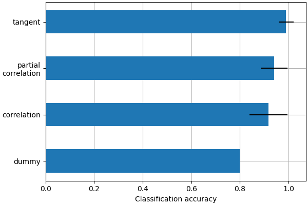
This is a small example to showcase nilearn features. In practice such comparisons need to be performed on much larger cohorts and several datasets. Dadi et al.[1] showed that across many cohorts and clinical questions, the tangent kind should be preferred.

plt.show()

References

[1] (1,2)

Kamalaker Dadi, Mehdi Rahim, Alexandre Abraham, Darya Chyzhyk, Michael Milham, Bertrand Thirion, and Gaël Varoquaux. Benchmarking functional connectome-based predictive models for resting-state fmri. NeuroImage, 192:115–134, 2019. URL: https://www.sciencedirect.com/science/article/pii/S1053811919301594, doi:https://doi.org/10.1016/j.neuroimage.2019.02.062.

Estimated memory usage: 1143 MB