10.1. Building your own neuroimaging machine-learning pipeline
Nilearn comes with code to simplify the use of scikit-learn when dealing with neuroimaging data. For the moment, nilearn is focused on functional MRI data.
Before using a machine learning tool, we may need to apply the following steps:
Data loading and preprocessing : load Nifti files and check consistency of data
Masking data : if a mask is not provided, one is computed automatically
Resampling images: optionally data could be resampled to a different resolution
Temporal Filtering and confound removal: detrending, regressing out confounds, normalization
10.1.1. Data loading and preprocessing
10.1.1.1. Downloading the data
To run demos, data are retrieved using a function provided by nilearn which downloads a dataset and returns a bunch of paths to the dataset files (more details in Inputing data: file names or image objects). We can then proceed loading them as if they were just any other files on our disk. For example, we can download the data from the Haxby 2001 paper :
from nilearn import datasets
dataset = datasets.fetch_haxby()
dataset.func contains filenames referring to dataset files on the disk:
list(sorted(dataset.keys()))
# ['anat', 'description', 'func', 'mask', 'mask_face', 'mask_face_little', 'mask_house', 'mask_house_little', 'mask_vt', 'session_target']
dataset.func
# ['.../haxby2001/subj2/bold.nii.gz']
Access supplementary information on the dataset:
print(haxby_dataset['description'])
The complete list of the data-downloading functions can be found in the reference documentation for the datasets.
10.1.1.2. Loading non image data: experiment description
An experiment may need additional information about subjects, sessions or experiments. In the Haxby experiment, fMRI data are acquired while presenting different category of pictures to the subject (face, cat, …) and the goal of this experiment is to predict which category is presented to the subjects from the brain activation.
These conditions are presented as string into a CSV file. The pandas function
read_csv is very useful to load this kind of data.
import pandas as pd

# Load behavioral information
behavioral = pd.read_csv(haxby_dataset.session_target[0], delimiter=" ")
print(behavioral)
See also
pandas is a very useful Python library to load CSV files and process their data
For example, we will now consider only the conditions cat and face from our dataset. This can be done as follows:
condition_mask = conditions.isin(["face", "cat"])
Note
If you are not comfortable with this kind of data processing, do not worry: there are plenty of examples in nilearn that allows you to easily load data from provided datasets. Do not hesitate to copy/paste the code and adapt it to your own data format if needed. More information can be found in the data manipulation section.
10.1.1.3. Masking the data: from 4D image to 2D array
While functional neuroimaging data consist in 4D images, positioned in a coordinate space (which we will call Niimgs). For use with the scikit-learn, they need to be converted into 2D arrays of samples and features.
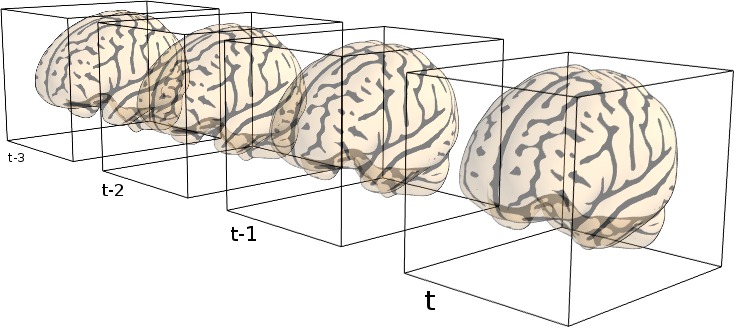 →
→ 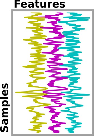
We use masking to convert 4D data (i.e. 3D volume over time) into 2D data
(i.e. voxels over time). For this purpose, we use the
NiftiMasker object, a very powerful data loading tool.
10.1.1.3.1. Applying a mask
If your dataset provides a mask, the NiftiMasker can apply it
automatically. All you have to do is to pass your mask as a parameter when
creating your masker. Here we use the mask of the ventral stream,
provided with the Haxby dataset.
The NiftiMasker can be seen as a tube that transforms data
from 4D images to 2D arrays, but first it needs to ‘fit’ this data in
order to learn simple parameters from it, such as its shape:
Warning
If you are using Nilearn with a version older than 0.9.0,
then you should either upgrade your version or import maskers
from the input_data module instead of the maskers module.
That is, you should manually replace in the following example all occurrences of:
from nilearn.maskers import NiftiMasker
with:
from nilearn.input_data import NiftiMasker
# We first create a masker, giving it the options that we care
# about. Here we use standardizing of the data, as it is often important
# for decoding
from nilearn.maskers import NiftiMasker

masker = NiftiMasker(mask_img=mask_filename, standardize=True)

# We give the masker a filename and retrieve a 2D array ready
# for machine learning with scikit-learn
fmri_masked = masker.fit_transform(fmri_filename)
Note that you can call nifti_masker.transform(dataset.func[1]) on new
data to mask it in a similar way as the data that was used during the
fit.
10.1.1.3.2. Automatically computing a mask
If your dataset does not provide a mask, the Nifti masker will compute
one for you in the fit step. The generated mask can be accessed via the
mask_img_ attribute.
Detailed information on automatic mask computation can be found in: Input and output: neuroimaging data representation.
10.1.2. Applying a scikit-learn machine learning method
Now that we have a 2D array, we can apply any estimator from the
scikit-learn, using its fit, predict or transform methods.
Here, we use scikit-learn Support Vector Classification to learn how to predict the category of picture seen by the subject:
svc.fit(fmri_masked, conditions)

###########################################################################
# We can then predict the labels from the data
prediction = svc.predict(fmri_masked)
print(prediction)

###########################################################################
We will not detail it here since there is a very good documentation about it in the scikit-learn documentation.
10.1.3. Unmasking (inverse_transform)
Unmasking data is as easy as masking it! This can be done by using
method inverse_transform on your processed data. As you may want to
unmask several kinds of data (not only the data that you previously
masked but also the results of an algorithm), the masker is clever and
can take data of dimension 1D (resp. 2D) to convert it back to 3D
(resp. 4D).
coef_img = masker.inverse_transform(coef_)
print(coef_img)
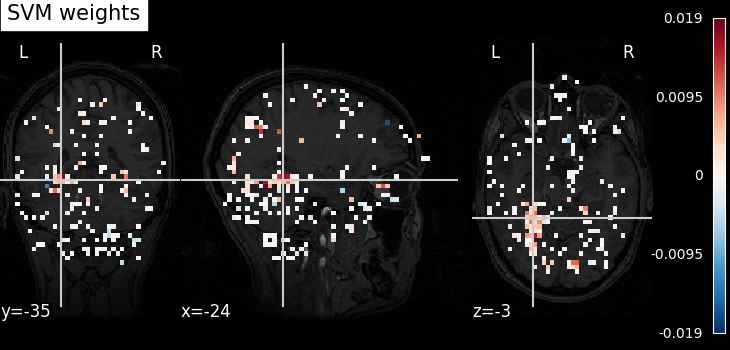
Here we want to see the discriminating weights of some voxels.
10.1.4. Visualizing results
Again the visualization code is simple. We can use an fMRI slice as a background and plot the weights. Brighter points have a higher discriminating weight.
from nilearn.plotting import plot_stat_map, show

plot_stat_map(
    coef_img, bg_img=haxby_dataset.anat[0], title="SVM weights", display_mode="yx"
)

show()
10.1.5. Going further
The NiftiMasker is a very powerful object and we have only
scratched the surface of its possibilities. It is described in more
details in the section NiftiMasker: applying a mask to load time-series. Also, simple functions that
can be used to perform elementary operations such as masking or filtering
are described in Functions for data preparation and image transformation.