6.1. Extracting times series to build a functional connectome
6.1.1. Time-series from a brain parcellation or “MaxProb” atlas
6.1.1.1. Brain parcellations
Regions used to extract the signal can be defined by a “hard”
parcellation. For instance, the nilearn.datasets has functions to
download atlases forming reference parcellation, e.g.,
fetch_atlas_craddock_2012, fetch_atlas_harvard_oxford,
fetch_atlas_yeo_2011.
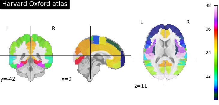
For instance to retrieve the Harvard-Oxford cortical parcellation, sampled at 2mm, and with a threshold of a probability of 0.25:
from nilearn import datasets
dataset = datasets.fetch_atlas_harvard_oxford('cort-maxprob-thr25-2mm')
atlas_filename = dataset.maps
labels = dataset.labels
Plotting can then be done as:
from nilearn import plotting
plotting.plot_roi(atlas_filename)
See also
The dataset downloaders.
6.1.1.2. Extracting signals on a parcellation
To extract signal on the parcellation, the easiest option is to use the
NiftiLabelsMasker. As any “maskers” in
nilearn, it is a processing object that is created by specifying all
the important parameters, but not the data:
from nilearn.maskers import NiftiLabelsMasker
masker = NiftiLabelsMasker(labels_img=atlas_filename, standardize=True)
The Nifti data can then be turned to time-series by calling the
NiftiLabelsMasker.fit_transform method, that takes either
filenames or NiftiImage objects:
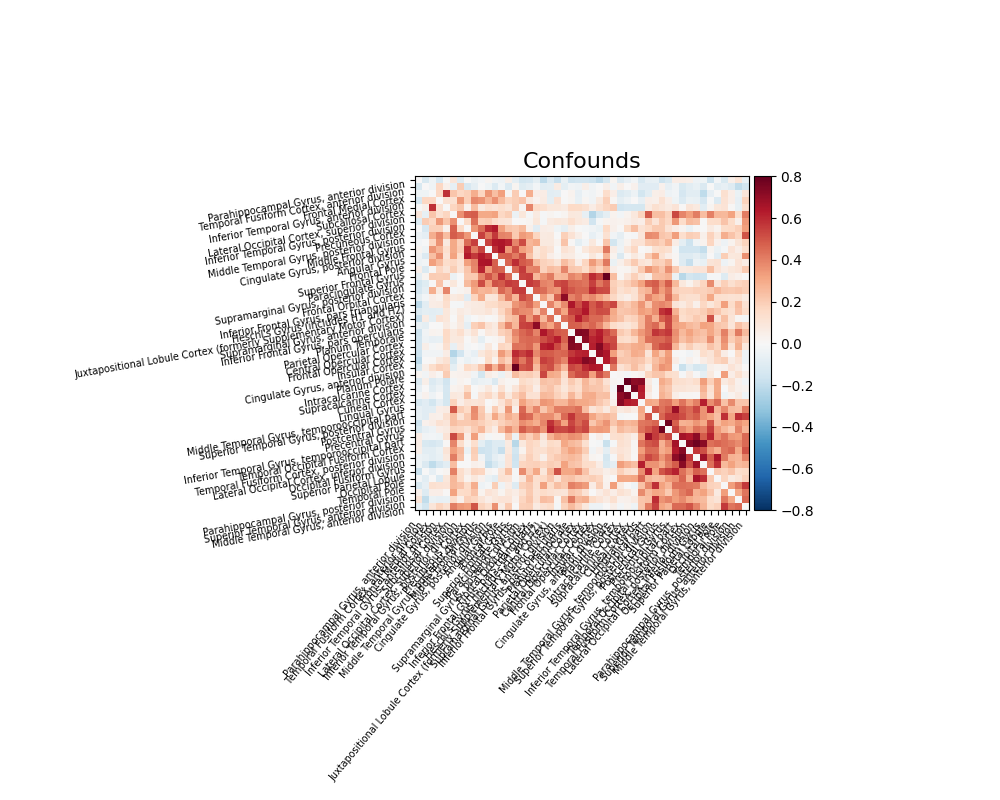
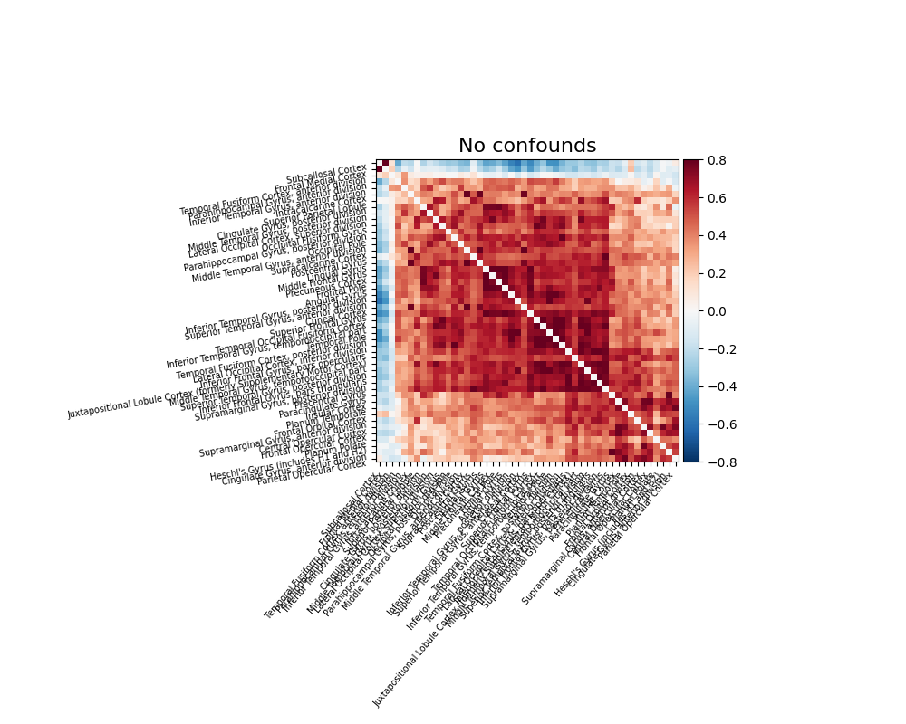
time_series = masker.fit_transform(frmi_files,
                                   confounds=confounds_dataframe)
Note that confound signals can be specified in the call. Indeed, to
obtain time series that capture well the functional interactions between
regions, regressing out noise sources is very important (Varoquaux and Craddock[1]).
For data processed by fMRIPrep,
load_confounds and
load_confounds_strategy can help you
retrieve confound variables.
load_confounds_strategy selects confounds
based on past literature with limited parameters for customization.
For more freedoms of confounds selection,
load_confounds groups confound variables as
sets of noise components and one can fine tune each of the parameters.
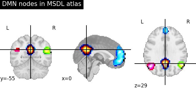
6.1.2. Time-series from a probabilistic atlas
6.1.2.1. Probabilistic atlases
The definition of regions as by a continuous probability map captures
better our imperfect knowledge of boundaries in brain images (notably
because of inter-subject registration errors). One example of such an
atlas well suited to resting-state or naturalistic-stimuli data analysis is
the MSDL atlas
(nilearn.datasets.fetch_atlas_msdl).
Probabilistic atlases are represented as a set of continuous maps, in a
4D nifti image. Visualization the atlas thus requires to visualize each
of these maps, which requires accessing them with
nilearn.image.index_img (see the corresponding example).
6.1.2.2. Extracting signals from a probabilistic atlas
As with extraction of signals on a parcellation, extracting signals from
a probabilistic atlas can be done with a “masker” object: the
NiftiMapsMasker. It is created by
specifying the important parameters, in particular the atlas:
from nilearn.maskers import NiftiMapsMasker
masker = NiftiMapsMasker(maps_img=atlas_filename, standardize=True)
The fit_transform method turns filenames or NiftiImage objects to time series:
time_series = masker.fit_transform(frmi_files, confounds=csv_file)
The procedure is the same as with brain parcellations
but using the NiftiMapsMasker, and
the same considerations on using confounds regressors apply.
6.1.3. A functional connectome: a graph of interactions
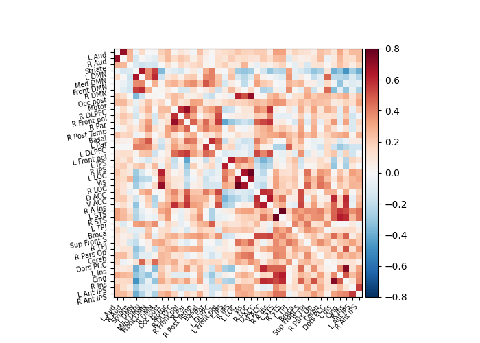
A square matrix, such as a correlation matrix, can also be seen as a “graph”: a set of “nodes”, connected by “edges”. When these nodes are brain regions, and the edges capture interactions between them, this graph is a “functional connectome”.
We can display it with the nilearn.plotting.plot_connectome
function that take the matrix, and coordinates of the nodes in MNI space.
In the case of the MSDL atlas
(nilearn.datasets.fetch_atlas_msdl), the CSV file readily comes
with MNI coordinates for each region (see for instance example:
Extracting signals of a probabilistic atlas of functional regions).
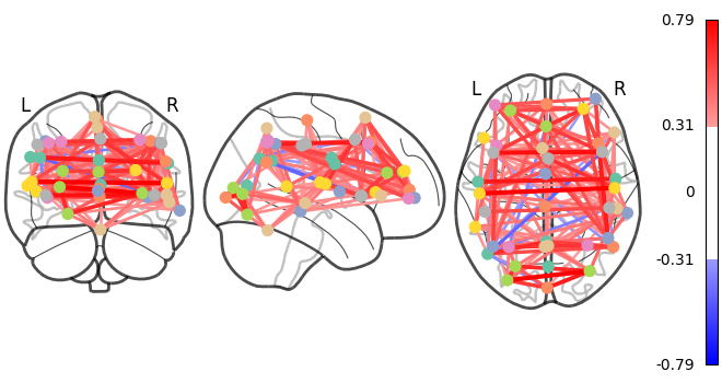
As you can see, the correlation matrix gives a very “full” graph: every node is connected to every other one. This is because it also captures indirect connections. In the next section we will see how to focus on direct connections only.
6.1.4. A functional connectome: extracting coordinates of regions
For atlases without readily available label coordinates, center coordinates can be computed for each region on hard parcellation or probabilistic atlases.
For hard parcellation atlases (eg.
nilearn.datasets.fetch_atlas_destrieux_2009), use thenilearn.plotting.find_parcellation_cut_coordsfunction. See example: Comparing connectomes on different reference atlasesFor probabilistic atlases (eg.
nilearn.datasets.fetch_atlas_msdl), use thenilearn.plotting.find_probabilistic_atlas_cut_coordsfunction. See example: Group Sparse inverse covariance for multi-subject connectome:
from nilearn import plotting

atlas_region_coords = plotting.find_probabilistic_atlas_cut_coords(atlas_filename)