Note
Go to the end to download the full example code. or to run this example in your browser via JupyterLite or Binder
Single-subject data (two runs) in native space
The example shows the analysis of an SPM dataset, with two conditions: viewing a face image or a scrambled face image.
This example takes a lot of time because the input are lists of 3D images sampled in different positions (encoded by different affine functions).
See also
For more information see the dataset description.
Fetch and inspect the data
Fetch the SPM multimodal_faces data.
from nilearn.datasets import fetch_spm_multimodal_fmri

subject_data = fetch_spm_multimodal_fmri()
[fetch_spm_multimodal_fmri] Dataset created in
/home/runner/nilearn_data/spm_multimodal_fmri
[fetch_spm_multimodal_fmri] Missing 390 functional scans for session 1.
[fetch_spm_multimodal_fmri] Data absent, downloading...
[fetch_spm_multimodal_fmri] Downloading data from
https://www.fil.ion.ucl.ac.uk/spm/download/data/mmfaces/multimodal_fmri.zip ...
[fetch_spm_multimodal_fmri] Downloaded 876544 of 134263085 bytes (0.7%%, 00 HR
02 MIN 50 SEC remaining)
[fetch_spm_multimodal_fmri] Downloaded 5136384 of 134263085 bytes (3.8%%, 00 HR
00 MIN 53 SEC remaining)
[fetch_spm_multimodal_fmri] Downloaded 12828672 of 134263085 bytes (9.6%%, 00 HR
00 MIN 30 SEC remaining)
[fetch_spm_multimodal_fmri] Downloaded 18300928 of 134263085 bytes (13.6%%, 00
HR 00 MIN 26 SEC remaining)
[fetch_spm_multimodal_fmri] Downloaded 23363584 of 134263085 bytes (17.4%%, 00
HR 00 MIN 24 SEC remaining)
[fetch_spm_multimodal_fmri] Downloaded 28688384 of 134263085 bytes (21.4%%, 00
HR 00 MIN 23 SEC remaining)
[fetch_spm_multimodal_fmri] Downloaded 34291712 of 134263085 bytes (25.5%%, 00
HR 00 MIN 21 SEC remaining)
[fetch_spm_multimodal_fmri] Downloaded 38690816 of 134263085 bytes (28.8%%, 00
HR 00 MIN 20 SEC remaining)
[fetch_spm_multimodal_fmri] Downloaded 43089920 of 134263085 bytes (32.1%%, 00
HR 00 MIN 20 SEC remaining)
[fetch_spm_multimodal_fmri] Downloaded 47775744 of 134263085 bytes (35.6%%, 00
HR 00 MIN 19 SEC remaining)
[fetch_spm_multimodal_fmri] Downloaded 52412416 of 134263085 bytes (39.0%%, 00
HR 00 MIN 18 SEC remaining)
[fetch_spm_multimodal_fmri] Downloaded 57163776 of 134263085 bytes (42.6%%, 00
HR 00 MIN 17 SEC remaining)
[fetch_spm_multimodal_fmri] Downloaded 61882368 of 134263085 bytes (46.1%%, 00
HR 00 MIN 16 SEC remaining)
[fetch_spm_multimodal_fmri] Downloaded 66674688 of 134263085 bytes (49.7%%, 00
HR 00 MIN 14 SEC remaining)
[fetch_spm_multimodal_fmri] Downloaded 71385088 of 134263085 bytes (53.2%%, 00
HR 00 MIN 13 SEC remaining)
[fetch_spm_multimodal_fmri] Downloaded 76308480 of 134263085 bytes (56.8%%, 00
HR 00 MIN 12 SEC remaining)
[fetch_spm_multimodal_fmri] Downloaded 81321984 of 134263085 bytes (60.6%%, 00
HR 00 MIN 11 SEC remaining)
[fetch_spm_multimodal_fmri] Downloaded 86237184 of 134263085 bytes (64.2%%, 00
HR 00 MIN 10 SEC remaining)
[fetch_spm_multimodal_fmri] Downloaded 91463680 of 134263085 bytes (68.1%%, 00
HR 00 MIN 09 SEC remaining)
[fetch_spm_multimodal_fmri] Downloaded 96894976 of 134263085 bytes (72.2%%, 00
HR 00 MIN 08 SEC remaining)
[fetch_spm_multimodal_fmri] Downloaded 102760448 of 134263085 bytes (76.5%%, 00
HR 00 MIN 07 SEC remaining)
[fetch_spm_multimodal_fmri] Downloaded 109191168 of 134263085 bytes (81.3%%, 00
HR 00 MIN 05 SEC remaining)
[fetch_spm_multimodal_fmri] Downloaded 114860032 of 134263085 bytes (85.5%%, 00
HR 00 MIN 04 SEC remaining)
[fetch_spm_multimodal_fmri] Downloaded 120553472 of 134263085 bytes (89.8%%, 00
HR 00 MIN 03 SEC remaining)
[fetch_spm_multimodal_fmri] Downloaded 125296640 of 134263085 bytes (93.3%%, 00
HR 00 MIN 02 SEC remaining)
[fetch_spm_multimodal_fmri] Downloaded 129835008 of 134263085 bytes (96.7%%, 00
HR 00 MIN 01 SEC remaining)
[fetch_spm_multimodal_fmri]  ...done. (28 seconds, 0 min)

[fetch_spm_multimodal_fmri] Extracting data from
/home/runner/nilearn_data/spm_multimodal_fmri/sub001/multimodal_fmri.zip...
[fetch_spm_multimodal_fmri] .. done.

[fetch_spm_multimodal_fmri] Downloading data from
https://www.fil.ion.ucl.ac.uk/spm/download/data/mmfaces/multimodal_smri.zip ...
[fetch_spm_multimodal_fmri] Downloaded 917504 of 6852766 bytes (13.4%%, 00 HR 00
MIN 07 SEC remaining)
[fetch_spm_multimodal_fmri] Downloaded 4923392 of 6852766 bytes (71.8%%, 00 HR
00 MIN 01 SEC remaining)
[fetch_spm_multimodal_fmri]  ...done. (3 seconds, 0 min)

[fetch_spm_multimodal_fmri] Extracting data from
/home/runner/nilearn_data/spm_multimodal_fmri/sub001/multimodal_smri.zip...
[fetch_spm_multimodal_fmri] .. done.
Let’s inspect one of the event files before using them.
import pandas as pd

events = [subject_data.events1, subject_data.events2]

events_dataframe = pd.read_csv(events[0], sep="\t")
events_dataframe["trial_type"].value_counts()
trial_type
scrambled    86
faces        64
Name: count, dtype: int64
We can confirm there are only 2 conditions in the dataset.
from nilearn.plotting import plot_event, show

plot_event(events)

show()
Resample the images:
this is achieved by the concat_imgs function of Nilearn.
import warnings

from nilearn.image import concat_imgs, mean_img, resample_img

# Avoid getting too many warnings due to resampling
with warnings.catch_warnings():
    warnings.simplefilter("ignore")
    fmri_img = [
        concat_imgs(subject_data.func1, auto_resample=True),
        concat_imgs(subject_data.func2, auto_resample=True),
    ]
affine, shape = fmri_img[0].affine, fmri_img[0].shape
print("Resampling the second image (this takes time)...")
fmri_img[1] = resample_img(fmri_img[1], affine, shape[:3])
Resampling the second image (this takes time)...
Let’s create mean image for display purposes.
Fit the model
Fit the GLM for the 2 runs by specifying a FirstLevelModel and then fitting it.
# Sample at the beginning of each acquisition.
slice_time_ref = 0.0
# We use a discrete cosine transform to model signal drifts.
drift_model = "cosine"
# The cutoff for the drift model is 0.01 Hz.
high_pass = 0.01
# The hemodynamic response function
hrf_model = "spm + derivative"

from nilearn.glm.first_level import FirstLevelModel

print("Fitting a GLM")
fmri_glm = FirstLevelModel(
    smoothing_fwhm=None,
    t_r=subject_data.t_r,
    hrf_model=hrf_model,
    drift_model=drift_model,
    high_pass=high_pass,
    verbose=1,
)


fmri_glm = fmri_glm.fit(fmri_img, events=events)
Fitting a GLM
\[FirstLevelModel.fit] Computing run 1 out of 2 runs (go take a coffee, a big
one).
\[FirstLevelModel.fit] Performing mask computation.
\[FirstLevelModel.fit] Masking took 0 seconds.
\[FirstLevelModel.fit] Performing GLM computation.
\[FirstLevelModel.fit] GLM took 1 seconds.
\[FirstLevelModel.fit] Computing run 2 out of 2 runs (00 HR 00 MIN 03 SEC
remaining).
\[FirstLevelModel.fit] Performing mask computation.
\[FirstLevelModel.fit] Masking took 0 seconds.
\[FirstLevelModel.fit] Performing GLM computation.
\[FirstLevelModel.fit] GLM took 1 seconds.
\[FirstLevelModel.fit] Computation of 2 runs done in 00 HR 00 MIN 04 SEC.
View the results
Now we can compute contrast-related statistical maps (in z-scale), and plot them.
from nilearn.plotting import plot_stat_map

print("Computing contrasts")
Computing contrasts
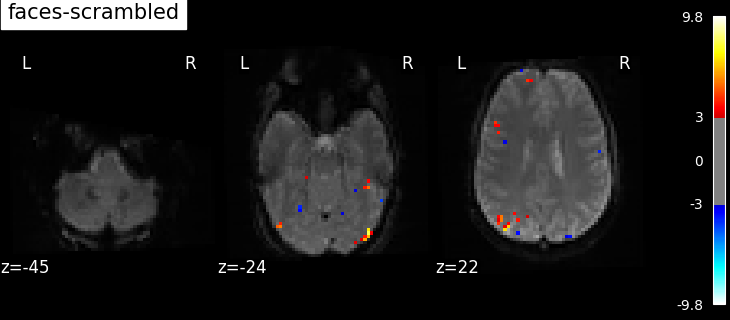
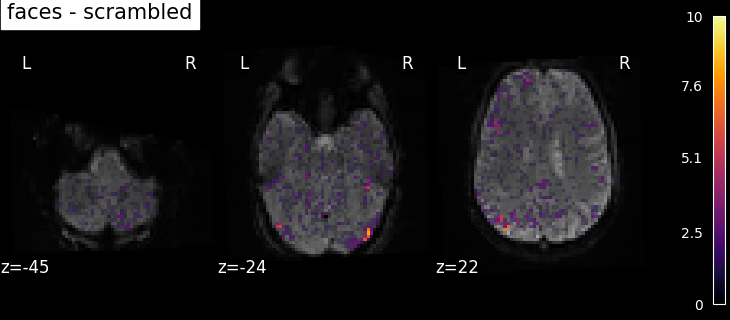
We actually want more interesting contrasts. The simplest contrast just makes the difference between the two main conditions. We define the two opposite versions to run one-tailed t-tests.
contrasts = ["faces - scrambled", "scrambled - faces"]
Let’s store common parameters for all plots.
We plot the contrasts values overlaid on the mean fMRI image and we will use the z-score values as transparency, with any voxel with | Z-score | > 3 being fully opaque and any voxel with 0 < | Z-score | < 1.96 being partly transparent.
plot_param = {
    "vmin": 0,
    "display_mode": "z",
    "cut_coords": 3,
    "black_bg": True,
    "bg_img": mean_image,
    "cmap": "inferno",
    "transparency_range": [0, 3],
}

# Iterate on contrasts to compute and plot them.
for contrast_id in contrasts:
    print(f"\tcontrast id: {contrast_id}")

    results = fmri_glm.compute_contrast(contrast_id, output_type="all")

    plot_stat_map(
        results["stat"],
        title=contrast_id,
        transparency=results["z_score"],
        **plot_param,
    )
        contrast id: faces - scrambled
/home/runner/work/nilearn/nilearn/examples/04_glm_first_level/plot_spm_multimodal_faces.py:134: RuntimeWarning:

The same contrast will be used for all 2 runs. If the design matrices are not the same for all runs, (for example with different column names or column order across runs) you should pass contrast as an expression using the name of the conditions as they appear in the design matrices.

        contrast id: scrambled - faces
/home/runner/work/nilearn/nilearn/examples/04_glm_first_level/plot_spm_multimodal_faces.py:134: RuntimeWarning:

The same contrast will be used for all 2 runs. If the design matrices are not the same for all runs, (for example with different column names or column order across runs) you should pass contrast as an expression using the name of the conditions as they appear in the design matrices.
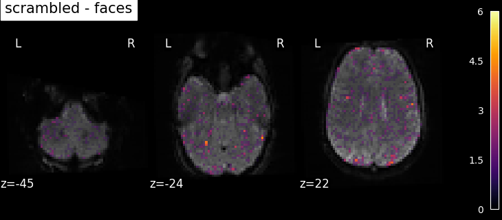
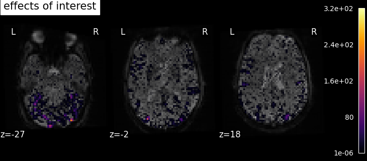
We also define the effects of interest contrast, a 2-dimensional contrasts spanning the two conditions.
import numpy as np

contrasts = np.eye(2)

results = fmri_glm.compute_contrast(contrasts, output_type="all")

plot_stat_map(
    results["stat"],
    title="effects of interest",
    transparency=results["z_score"],
    **plot_param,
)

show()
/home/runner/work/nilearn/nilearn/examples/04_glm_first_level/plot_spm_multimodal_faces.py:151: RuntimeWarning:

The same contrast will be used for all 2 runs. If the design matrices are not the same for all runs, (for example with different column names or column order across runs) you should pass contrast as an expression using the name of the conditions as they appear in the design matrices.

/home/runner/work/nilearn/nilearn/examples/04_glm_first_level/plot_spm_multimodal_faces.py:151: UserWarning:

F contrasts should have 20 columns, but it has only 2. The rest of the contrast was padded with zeros.

/home/runner/work/nilearn/nilearn/examples/04_glm_first_level/plot_spm_multimodal_faces.py:151: UserWarning:

Running approximate fixed effects on F statistics.
Based on the resulting maps we observe that the analysis results in wide activity for the ‘effects of interest’ contrast, showing the implications of large portions of the visual cortex in the conditions. By contrast, the differential effect between “faces” and “scrambled” involves sparser, more anterior and lateral regions. It also displays some responses in the frontal lobe.
Total running time of the script: (1 minutes 50.555 seconds)
Estimated memory usage: 1059 MB