Example of MRI response functions

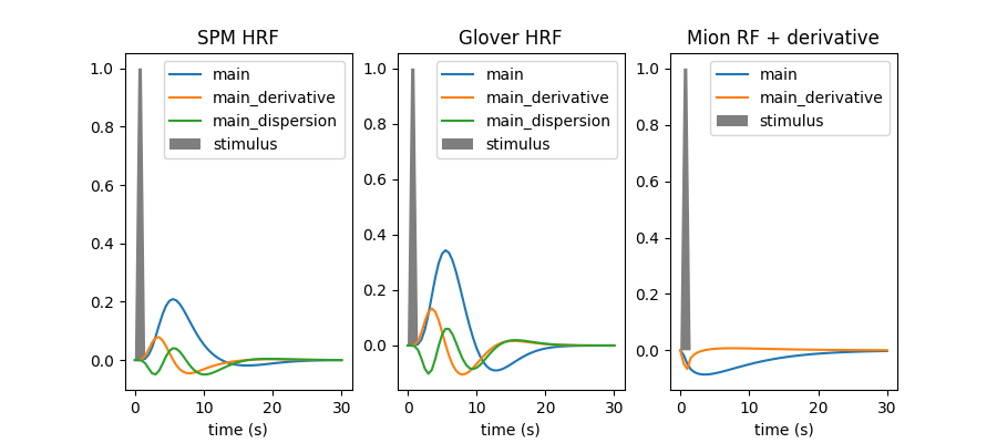
Within this example we are going to plot the hemodynamic response function (HRF) model in SPM together with the HRF shape proposed by G.Glover, as well as their time and dispersion derivatives. We also illustrate how users can input a custom response function, which can for instance be useful when dealing with non human primate data acquired using a contrast agent. In our case, we input a custom response function for MION, a common agent used to enhance contrast on MRI images of monkeys.

The HRF is the filter which couples neural responses to the metabolic-related changes in the MRI signal. HRF models are simply phenomenological.

In current analysis frameworks, the choice of HRF model is essentially left to the user. Fortunately, using the SPM or Glover model does not make a huge difference. Adding derivatives should be considered whenever timing information has some degree of uncertainty, and is actually useful to detect timing issues.

This example requires matplotlib and scipy.

from nilearn._utils.helpers import check_matplotlib

check_matplotlib()

import matplotlib.pyplot as plt
import numpy as np

Define stimulus parameters and response models

To get an impulse response, we simulate a single event occurring at time t=0, with duration 1s.

time_length = 30.0
frame_times = np.linspace(0, time_length, 61)
onset, amplitude, duration = 0.0, 1.0, 1.0
exp_condition = np.array((onset, duration, amplitude)).reshape(3, 1)

Make a time array of this condition for display:

stim = np.zeros_like(frame_times)
stim[(frame_times > onset) * (frame_times <= onset + duration)] = amplitude

Define custom response functions for MION. Custom response functions should at least take TR and oversampling as arguments:

from scipy.stats import gamma


def mion_response_function(t_r, oversampling=16, onset=0.0):
    """Implement the MION response function model.

    Parameters
    ----------
    t_r : float
        scan repeat time, in seconds
    oversampling : int, optional
        temporal oversampling factor
    onset : float, optional
        hrf onset time, in seconds

    Returns
    -------
    response_function :
        array of shape(length / t_r * oversampling, dtype=float)
        response_function sampling on the oversampled time grid
    """
    dt = t_r / oversampling
    time_stamps = np.linspace(
        0, time_length, np.rint(time_length / dt).astype(int)
    )
    time_stamps -= onset

    # parameters of the gamma function
    delay = 1.55
    dispersion = 5.5

    response_function = gamma.pdf(time_stamps, delay, loc=0, scale=dispersion)
    response_function /= response_function.sum()
    response_function *= -1

    return response_function


def mion_time_derivative(t_r, oversampling=16.0):
    """Implement the MION time derivative response function model.

    Parameters
    ----------
    t_r : float
        scan repeat time, in seconds
    oversampling : int, optional
        temporal oversampling factor, optional

    Returns
    -------
    drf : array of shape(time_length / t_r * oversampling, dtype=float)
        derived_response_function sampling on the provided grid
    """
    do = 0.1
    drf = (
        mion_response_function(t_r, oversampling)
        - mion_response_function(t_r, oversampling, do)
    ) / do

    return drf

Define response function models to be displayed:

rf_models = [
    ("spm + derivative + dispersion", "SPM HRF", None),
    ("glover + derivative + dispersion", "Glover HRF", None),
    (
        [mion_response_function, mion_time_derivative],
        "Mion RF + derivative",
        ["main", "main_derivative"],
    ),
]

Sample and plot response functions

from nilearn.glm.first_level import compute_regressor

oversampling = 16

fig = plt.figure(figsize=(9, 4))
for i, (rf_model, model_title, labels) in enumerate(rf_models):
    # compute signal of interest by convolution
    signal, _labels = compute_regressor(
        exp_condition,
        rf_model,
        frame_times,
        con_id="main",
        oversampling=oversampling,
    )

    # plot signal
    plt.subplot(1, len(rf_models), i + 1)
    plt.fill(frame_times, stim, "k", alpha=0.5, label="stimulus")
    for j in range(signal.shape[1]):
        plt.plot(
            frame_times,
            signal.T[j],
            label=(
                labels[j]
                if labels is not None
                else (_labels[j] if _labels is not None else None)
            ),
        )
    plt.xlabel("time (s)")
    plt.legend(loc=1)
    plt.title(model_title)

# adjust plot
plt.subplots_adjust(bottom=0.12)
plt.show()

Estimated memory usage: 146 MB