6.5. Clustering to parcellate the brain in regions

This page discusses how clustering can be used to parcellate the brain into homogeneous regions from functional imaging data.

Reference

A big-picture reference on the use of clustering for brain parcellations can be found in Thirion et al.[1].

6.5.1. Data loading: movie-watching data

Clustering is commonly applied to resting-state data, but any brain functional data will give rise of a functional parcellation, capturing intrinsic brain architecture in the case of resting-state data. In the examples, we use naturalistic stimuli-based movie watching brain development data downloaded with the function fetch_development_fmri (see Inputing data: file names or image objects).

6.5.2. Applying clustering

Which clustering to use

The question of which clustering method to use is in itself subject to debate. There are many clustering methods; their computational cost will vary, as well as their results. A well-cited empirical comparison paper (Thirion et al.[1]) suggests that:

• For a large number of clusters, it is preferable to use Ward agglomerative clustering with spatial constraints

• For a small number of clusters, it is preferable to use Kmeans clustering after spatially-smoothing the data.

Both algorithms are provided by this object nilearn.regions.Parcellations as well as two algorithms tailored to more specific usecases:

• nilearn.regions.ReNA is a quicker alternative to Ward with a small loss of precision, it is ideal to downsize the number of voxels by 10 quickly.

• Hierarchical KMeans is useful to obtain a small number of clusters after spatial smoothing, that will be better balanced than with Kmeans.

All these algorithms are showcased in a full code example : here. Below, we focus on explaining the principle of Ward.

Compute a connectivity matrix Before applying Ward’s method, we compute a spatial neighborhood matrix, aka connectivity matrix. This is useful to constrain clusters to form contiguous parcels (see the scikit-learn documentation)

This is done from the mask computed by the masker: a niimg from which we extract a numpy array and then the connectivity matrix.

Ward clustering principle Ward’s algorithm is a hierarchical clustering algorithm: it recursively merges voxels, then clusters that have similar signal (parameters, measurements or time courses).

Caching In practice the implementation of Ward clustering first computes a tree of possible merges, and then, given a requested number of clusters, breaks apart the tree at the right level.

As the tree is independent of the number of clusters, we can rely on caching to speed things up when varying the number of clusters. In Wards clustering, the memory parameter is used to cache the computed component tree. You can give it either a joblib.Memory instance or the name of a directory used for caching.

Note

The Ward clustering computing 1000 parcels runs typically in about 10 seconds. Admittedly, this is very fast.

Note

The steps detailed above such as computing connectivity matrix for Ward, caching and clustering are all implemented within the nilearn.regions.Parcellations object.

See also

• A function nilearn.regions.connected_label_regions which can be useful to break down connected components into regions. For instance, clusters defined using KMeans whereas it is not necessary for Ward clustering due to its spatial connectivity.

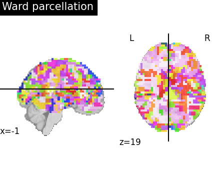
6.5.3. Using and visualizing the resulting parcellation

6.5.3.1. Visualizing the parcellation

The labels of the parcellation are found in the labels_img_ attribute of the nilearn.regions.Parcellations object after fitting it to the data using ward.fit. We directly use the result for visualization.

To visualize the clusters, we assign random colors to each cluster for the labels visualization.

6.5.3.2. Compressed representation

The clustering can be used to transform the data into a smaller representation, taking the average on each parcel:

• call ward.transform to obtain the mean value of each cluster (for each scan)

• call ward.inverse_transform on the previous result to turn it back into the masked picture shape

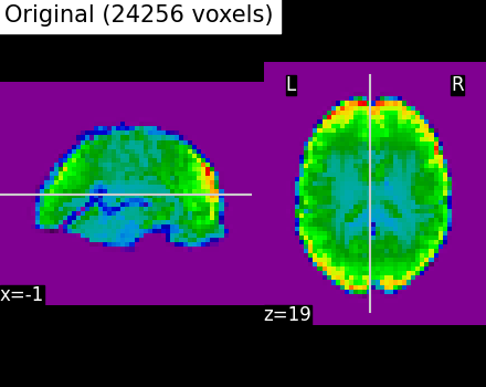
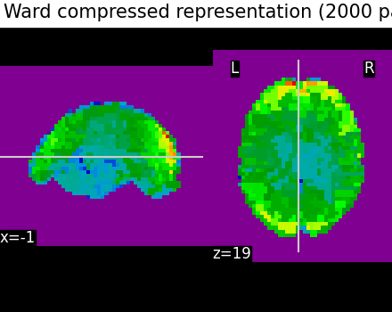
We can see that using only 2000 parcels, the original image is well approximated.

Example code

All the steps discussed in this section can be seen implemented in a full code example.

6.5.3.3. References

[1] (1,2)

Bertrand Thirion, Gaël Varoquaux, Elvis Dohmatob, and Jean-Baptiste Poline. Which fmri clustering gives good brain parcellations? Frontiers in Neuroscience, 2014. URL: https://www.frontiersin.org/articles/10.3389/fnins.2014.00167, doi:10.3389/fnins.2014.00167.