Note
Go to the end to download the full example code. or to run this example in your browser via JupyterLite or Binder
Example of surface-based first-level analysis
A full step-by-step example of fitting a GLM to experimental data sampled on the cortical surface and visualizing the results.
More specifically:
A sequence of fMRI volumes is loaded.
fMRI data are projected onto a reference cortical surface (the FreeSurfer template, fsaverage).
A GLM is applied to the dataset (effect/covariance, then contrast estimation).
Inspect GLM reports and save the results to disk.
The results of the analysis are statistical maps that are defined on the brain mesh. We display them using Nilearn capabilities.
The projection of fMRI data onto a given brain mesh requires that both are initially defined in the same space.
The functional data should be coregistered to the anatomy from which the mesh was obtained.
Another possibility, used here, is to project the normalized fMRI data to an MNI-coregistered mesh, such as fsaverage.
The advantage of this second approach is that it makes it easy to run second-level analyses on the surface. On the other hand, it is obviously less accurate than using a subject-tailored mesh.
See also
For more information about the dataset see its description.
Prepare data and analysis parameters
Fetch the data.
from nilearn.datasets import fetch_localizer_first_level

data = fetch_localizer_first_level()
t_r = data.t_r
slice_time_ref = data.slice_time_ref
[fetch_localizer_first_level] Dataset directory found:
/home/runner/nilearn_data/localizer_first_level
Project the fMRI image to the surface
For this we need to get a mesh representing the geometry of the surface. We could use an individual mesh, but we first resort to a standard mesh, the so-called fsaverage5 template from the FreeSurfer software.
We use the SurfaceImage
to create an surface object instance
that contains both the mesh
(here we use the one from the fsaverage5 templates)
and the BOLD data that we project on the surface.
from nilearn.datasets import load_fsaverage
from nilearn.surface import SurfaceImage

fsaverage5 = load_fsaverage()
surface_image = SurfaceImage.from_volume(
    mesh=fsaverage5["pial"],
    volume_img=data.epi_img,
)
Perform first level analysis
We can now simply run a GLM by directly passing
our SurfaceImage instance
as input to FirstLevelModel.fit
Here we use an HRF model containing the Glover model and its time derivative The drift model is implicitly a cosine basis with a period cutoff at 128s.
from nilearn.glm.first_level import FirstLevelModel

glm = FirstLevelModel(
    t_r=t_r,
    slice_time_ref=slice_time_ref,
    hrf_model="glover + derivative",
    minimize_memory=False,
    smoothing_fwhm=4,
    verbose=1,
).fit(run_imgs=surface_image, events=data.events)
\[FirstLevelModel.fit] Computing run 1 out of 1 runs (go take a coffee, a big
one).
\[FirstLevelModel.fit] Performing mask computation.
\[FirstLevelModel.fit] Masking took 0 seconds.
\[FirstLevelModel.fit] Performing GLM computation.
\[FirstLevelModel.fit] GLM took 0 seconds.
\[FirstLevelModel.fit] Computation of 1 runs done in 00 HR 00 MIN 01 SEC.
Estimate contrasts
Specify the contrasts.
For practical purpose, we first generate an identity matrix whose size is the number of columns of the design matrix.
import numpy as np

design_matrix = glm.design_matrices_[0]
contrast_matrix = np.eye(design_matrix.shape[1])
At first, we create basic contrasts.
basic_contrasts = {
    column: contrast_matrix[i]
    for i, column in enumerate(design_matrix.columns)
}
Next, we add some intermediate contrasts and one contrast adding all conditions with some auditory parts.
basic_contrasts["audio"] = (
    basic_contrasts["audio_left_hand_button_press"]
    + basic_contrasts["audio_right_hand_button_press"]
    + basic_contrasts["audio_computation"]
    + basic_contrasts["sentence_listening"]
)
one contrast adding all conditions involving instructions reading
basic_contrasts["visual"] = (
    basic_contrasts["visual_left_hand_button_press"]
    + basic_contrasts["visual_right_hand_button_press"]
    + basic_contrasts["visual_computation"]
    + basic_contrasts["sentence_reading"]
)
one contrast adding all conditions involving computation
basic_contrasts["computation"] = (
    basic_contrasts["visual_computation"]
    + basic_contrasts["audio_computation"]
)
one contrast adding all conditions involving sentences
basic_contrasts["sentences"] = (
    basic_contrasts["sentence_listening"] + basic_contrasts["sentence_reading"]
)
Finally, we create a dictionary of more relevant contrasts
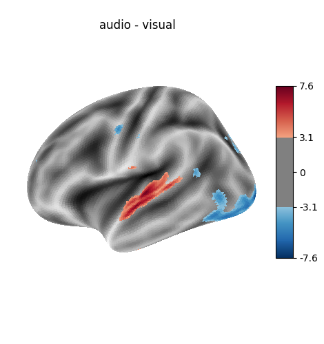
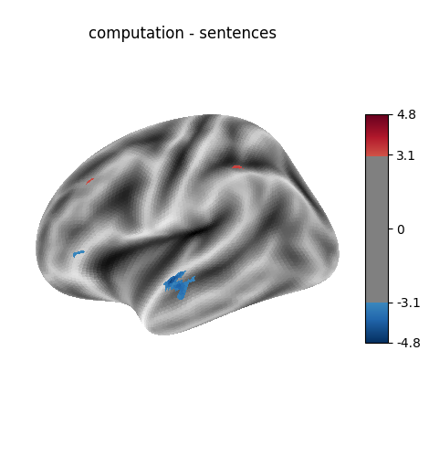
'left - right button press': probes motor activity in left versus right button presses.'audio - visual': probes the difference of activity between listening to some content or reading the same type of content (instructions, stories).'computation - sentences': looks at the activity when performing a mental computation task versus simply reading sentences.
Of course, we could define other contrasts, but we keep only 3 for simplicity.
contrasts = {
    "(left - right) button press": (
        basic_contrasts["audio_left_hand_button_press"]
        - basic_contrasts["audio_right_hand_button_press"]
        + basic_contrasts["visual_left_hand_button_press"]
        - basic_contrasts["visual_right_hand_button_press"]
    ),
    "audio - visual": basic_contrasts["audio"] - basic_contrasts["visual"],
    "computation - sentences": (
        basic_contrasts["computation"] - basic_contrasts["sentences"]
    ),
}
Let’s estimate the t-contrasts, and extract a table of clusters that survive our thresholds.
We use the same threshold (uncorrected p < 0.001) for all contrasts.
We plot each contrast map on the inflated fsaverage mesh, together with a suitable background to give an impression of the cortex folding.
from scipy.stats import norm
from nilearn.datasets import load_fsaverage_data
from nilearn.plotting import plot_surf_stat_map, show
from nilearn.reporting import get_clusters_table
p_val = 0.001
threshold = norm.isf(p_val)
cluster_threshold = 20
two_sided = True
fsaverage_data = load_fsaverage_data(data_type="sulcal")
results = {}
for contrast_id, contrast_val in contrasts.items():
results[contrast_id] = glm.compute_contrast(contrast_val, stat_type="t")
table = get_clusters_table(
results[contrast_id],
stat_threshold=threshold,
cluster_threshold=cluster_threshold,
two_sided=two_sided,
)
print(f"\n{contrast_id=}")
print(table)
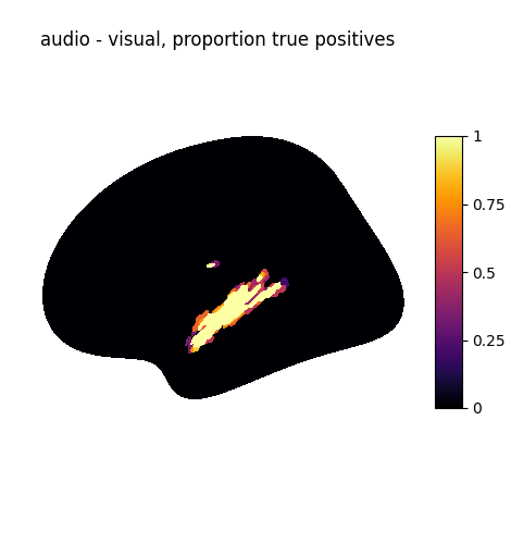
for contrast_id, z_score in results.items():
hemi = "left"
if contrast_id == "(left - right) button press":
hemi = "both"
plot_surf_stat_map(
surf_mesh=fsaverage5["inflated"],
stat_map=z_score,
hemi=hemi,
title=contrast_id,
threshold=threshold,
bg_map=fsaverage_data,
)
show()
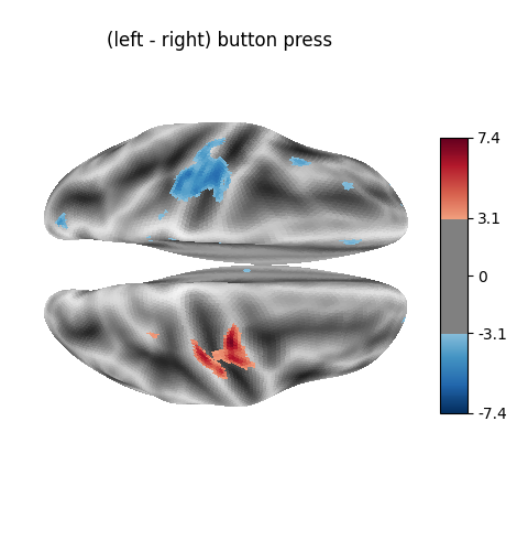
contrast_id='(left - right) button press'
  Cluster ID Hemisphere  Peak Stat  Cluster Size (vertices)
0          1      right   7.619268                      150
1          2       left  -3.094002                      245
2          3       left  -3.115826                       24
3          4       left  -3.101529                       24

contrast_id='audio - visual'
  Cluster ID Hemisphere  Peak Stat  Cluster Size (vertices)
0          1       left   7.541723                      203
1          2      right   7.499746                      162
2          3      right   6.289434                       78
3          4       left  -3.090704                      253
4          5       left  -3.100321                       72
5          6       left  -3.090740                       21
6          7      right  -3.107054                      143
7          8      right  -3.094296                       33
8          9      right  -3.092160                      293
9         10      right  -3.093588                       53

contrast_id='computation - sentences'
  Cluster ID Hemisphere  Peak Stat  Cluster Size (vertices)
0          1      right   3.774950                       34
1          2       left  -3.093961                       52
Cluster-level inference
We can also perform cluster-level inference (aka “All resolution Inference”) for a given contrast. This gives a high-probability lower bound on the proportion of true discoveries in each cluster
from nilearn.glm import cluster_level_inference
from nilearn.surface.surface import get_data as get_surf_data

proportion_true_discoveries_img = cluster_level_inference(
    results["audio - visual"], threshold=[2.5, 3.5, 4.5], alpha=0.05
)

data = get_surf_data(proportion_true_discoveries_img)
unique_vals = np.unique(data.ravel())
print(unique_vals)

plot_surf_stat_map(
    surf_mesh=fsaverage5["inflated"],
    stat_map=proportion_true_discoveries_img,
    hemi="left",
    cmap="inferno",
    title="audio - visual, proportion true positives",
    bg_map=fsaverage_data,
    avg_method="max",
)

show()
[-0.          0.2         0.25        0.33333333  0.38461538  0.4
  0.42857143  0.4375      0.45        0.5         0.53846154  0.55555556
  0.57142857  0.6         0.625       0.63636364  0.66666667  0.69230769
  0.69565217  0.71428571  0.75        0.8         0.81818182  0.83333333
  0.84615385  0.85714286  0.875       0.9         0.91666667  1.        ]
Generate a report for the GLM
report = glm.generate_report(
    contrasts,
    threshold=threshold,
    bg_img=load_fsaverage_data(data_type="sulcal", mesh_type="inflated"),
    height_control=None,
    cluster_threshold=cluster_threshold,
    two_sided=two_sided,
)
/home/runner/work/nilearn/nilearn/examples/04_glm_first_level/plot_localizer_surface_analysis.py:275: RuntimeWarning:

Meshes are not identical but have compatible number of vertices.

/home/runner/work/nilearn/nilearn/examples/04_glm_first_level/plot_localizer_surface_analysis.py:275: RuntimeWarning:

Meshes are not identical but have compatible number of vertices.

/home/runner/work/nilearn/nilearn/examples/04_glm_first_level/plot_localizer_surface_analysis.py:275: RuntimeWarning:

Meshes are not identical but have compatible number of vertices.
Note
The generated report can be:
displayed in a Notebook,
opened in a browser using the
.open_in_browser()method,or saved to a file using the
.save_as_html(output_filepath)method.
FirstLevelModel Implement the General Linear Model for single run :term:`fMRI` data.
Description
Data were analyzed using Nilearn (version= 0.14.0; RRID:SCR_001362).
At the subject level, a mass univariate analysis was performed with a linear regression at each voxel of the brain, using generalized least squares with a global ar1 noise model to account for temporal auto-correlation and a cosine drift model (high pass filter=0.01 Hz).
Regressors were entered into run-specific design matrices and onsets were convolved with a glover + derivative canonical hemodynamic response function for the following conditions:
- audio_computation
- audio_left_hand_button_press
- audio_right_hand_button_press
- horizontal_checkerboard
- sentence_listening
- sentence_reading
- vertical_checkerboard
- visual_computation
- visual_left_hand_button_press
- visual_right_hand_button_press
Input images were smoothed with gaussian kernel (full-width at half maximum=4 mm).
Model details
| Value | |
|---|---|
| Parameter | |
| drift_model | cosine |
| high_pass (Hertz) | 0.01 |
| hrf_model | glover + derivative |
| noise_model | ar1 |
| signal_scaling | 0 |
| slice_time_ref | 0.5 |
| smoothing_fwhm (mm) | 4 |
| standardize | False |
| t_r (seconds) | 2.4 |
Design Matrix

correlation matrix

Contrasts
 button press (run 0).")
.")
.")
Mask

The mask includes 20484 voxels (100.0 %) of the image.
Statistical Maps
(left - right) button press
 button press")
Cluster Table
| Height control | None |
|---|---|
| Threshold Z | 3.09 |
| Cluster ID | Hemisphere | Peak Stat | Cluster Size (vertices) |
|---|---|---|---|
| 1 | right | 7.62 | 150 |
| 2 | left | -3.09 | 245 |
| 3 | left | -3.12 | 24 |
| 4 | left | -3.10 | 24 |
audio - visual

Cluster Table
| Height control | None |
|---|---|
| Threshold Z | 3.09 |
| Cluster ID | Hemisphere | Peak Stat | Cluster Size (vertices) |
|---|---|---|---|
| 1 | left | 7.54 | 203 |
| 2 | right | 7.50 | 162 |
| 3 | right | 6.29 | 78 |
| 4 | left | -3.09 | 253 |
| 5 | left | -3.10 | 72 |
| 6 | left | -3.09 | 21 |
| 7 | right | -3.11 | 143 |
| 8 | right | -3.09 | 33 |
| 9 | right | -3.09 | 293 |
| 10 | right | -3.09 | 53 |
computation - sentences

Cluster Table
| Height control | None |
|---|---|
| Threshold Z | 3.09 |
| Cluster ID | Hemisphere | Peak Stat | Cluster Size (vertices) |
|---|---|---|---|
| 1 | right | 3.77 | 34 |
| 2 | left | -3.09 | 52 |
About
- Date preprocessed:
Total running time of the script: (0 minutes 31.940 seconds)
Estimated memory usage: 345 MB