Note
Go to the end to download the full example code. or to run this example in your browser via JupyterLite or Binder
More plotting tools from nilearn
In this example, we show how to use some plotting options available with plotting functions of nilearn. These techniques are essential for visualizing brain image analysis results.
Plotting functions of Nilearn, such as
plot_stat_map, have a few useful parameters
which control what type of display object will be
returned, as well as how many cuts will be shown for example.
As we will see in the first part of this example, depending on the values of
the parameters display_mode and cut_coords, plotting functions return
different display objects, all subclasses of
OrthoSlicer.
These objects implement various methods to interact with the figures. In the
second part of this example, we show how to use these methods to further
customize the figures obtained with plotting functions. More precisely, we
will show how to use add_edges,
add_contours, and
add_markers, all essential
in visualizing regions of interest images, or mask images overlaying on
subject specific anatomical / EPI image.
The parameter display_mode is used to draw brain slices along given
specific directions, where directions can be one of ‘ortho’,
‘tiled’, ‘mosaic’, ‘x’, ‘y’, ‘z’, ‘yx’, ‘xz’, ‘yz’. Whereas parameter
cut_coords is used to specify a limited number of slices to visualize
along given specific slice direction.
The parameter cut_coords can also be used to draw the specific cuts in
the slices by giving its particular coordinates in MNI space
accordingly with particular slice direction. This helps us point to the
activation specific location of the brain slices.
See Plotting brain images for more details.
Display objects returned by plotting functions
Plotting functions return different display objects depending on the values
of the parameters display_mode and cut_coords.
We first retrieve data from nilearn provided (general-purpose) datasets.
from nilearn import datasets

# haxby dataset to have anatomical image, EPI images and masks
haxby_dataset = datasets.fetch_haxby()
haxby_anat_filename = haxby_dataset.anat[0]
haxby_mask_filename = haxby_dataset.mask_vt[0]
haxby_func_filename = haxby_dataset.func[0]

# example motor activation image distributed with nilearn
stat_img = datasets.load_sample_motor_activation_image()
[fetch_haxby] Dataset directory found: /home/runner/nilearn_data/haxby2001
Now, we show from here how to visualize the retrieved datasets using plotting tools from nilearn.
from nilearn import plotting
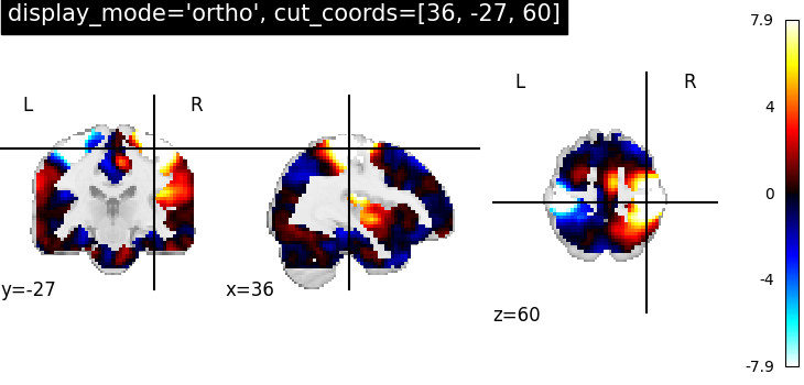
OrthoSlicer: Three views ‘sagittal’, ‘coronal’ and ‘axial’ with coordinates
The first argument stat_img is a path to the filename of a contrast map.
The optional argument display_mode is given as a string ‘ortho’ to
visualize the map in three specific directions xyz. Because of this, the
plotting function returns a OrthoSlicer
object. The optional cut_coords argument is specified here as a list of
integers representing coordinates of each slice in the order [x, y, z].
By default the colorbar argument is set to True in
plot_stat_map.
plotting.plot_stat_map(
    stat_img,
    display_mode="ortho",
    cut_coords=[36, -27, 60],
    title="display_mode='ortho', cut_coords=[36, -27, 60]",
)
<nilearn.plotting.displays._slicers.OrthoSlicer object at 0x7f0c02415e70>
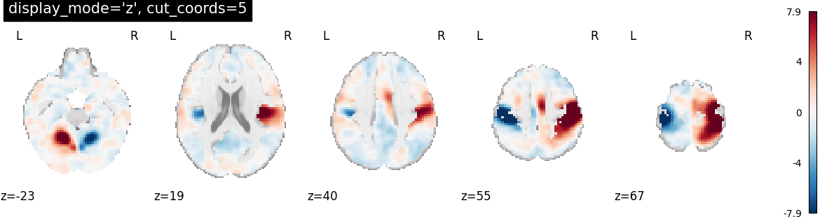
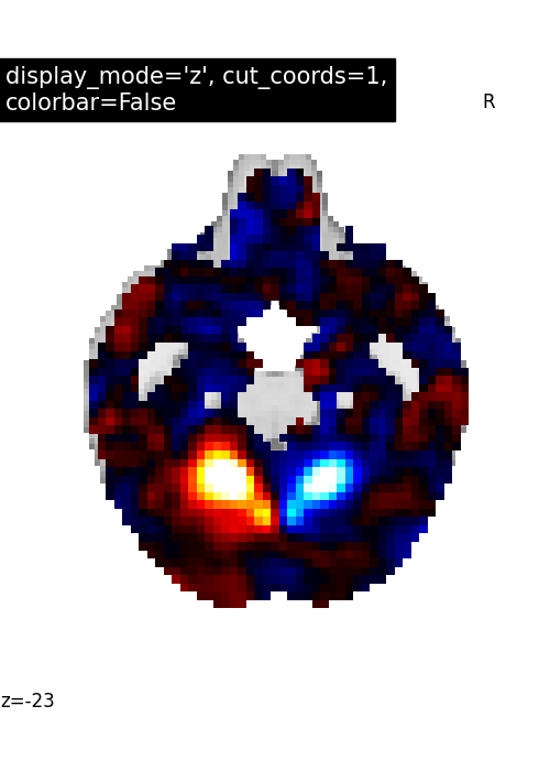
ZSlicer: Single view ‘axial’ with number of cuts=5
For axial visualization, we set display_mode='z'. As a
consequence plot_stat_map returns a
ZSlicer object.
The parameter cut_coords is provided here as an integer (5) rather than
a list, which implies that the number of cuts in the slices should be 5
maximum. Note that the coordinates used to cut the slices are selected
automatically.
plotting.plot_stat_map(
    stat_img,
    display_mode="z",
    cut_coords=5,
    title="display_mode='z', cut_coords=5",
)
<nilearn.plotting.displays._slicers.ZSlicer object at 0x7f0c03a1aad0>
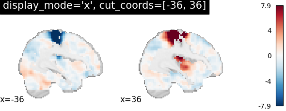
XSlicer: Single view ‘sagittal’ with only two slices
For sagittal visualization, we set display_mode='x' which returns a
XSlicer object.
Additionally, we provide the coordinates of the slices as a list of
integers.
plotting.plot_stat_map(
    stat_img,
    display_mode="x",
    cut_coords=[-36, 36],
    title="display_mode='x', cut_coords=[-36, 36]",
)
<nilearn.plotting.displays._slicers.XSlicer object at 0x7f0bf2f279d0>
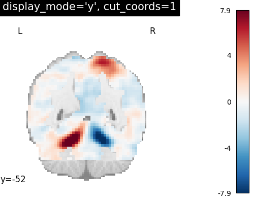
YSlicer: Single view ‘coronal’ with single cut
For coronal view, we set display_mode='y' which returns a
YSlicer object.
cut_coords is provided as an integer (1), and the coordinates are,
again, selected automatically.
import matplotlib.pyplot as plt

plotting.plot_stat_map(
    stat_img,
    display_mode="y",
    cut_coords=1,
    title="display_mode='y', cut_coords=1",
    figure=plt.figure(figsize=(5, 4)),
)
<nilearn.plotting.displays._slicers.YSlicer object at 0x7f0c18b79360>
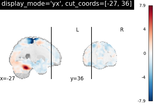
XZSlicer: Two views ‘sagittal’ and ‘axial’ with given coordinates
In order to visualize both sagittal and axial views, we set
display_mode='xz', where ‘x’ stands for sagittal and ‘z’ for axial view.
Function plot_stat_map thus returns a
XZSlicer object.
Finally, the argument cut_coords should match with the input number of
views (two here). It is provided as a list of integers here to select the
slices to be displayed.
plotting.plot_stat_map(
    stat_img,
    display_mode="xz",
    cut_coords=[36, 60],
    title="display_mode='xz', cut_coords=[36, 60]",
)
<nilearn.plotting.displays._slicers.XZSlicer object at 0x7f0c1c41b1c0>
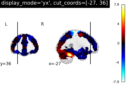
YXSlicer: Two views ‘coronal’ and ‘sagittal’ with coordinates
Similarly, we can set display_mode='yx' for combining a coronal with a
sagittal view, which will return a
YXSlicer object.
The coordinates will be assigned in the order of direction as [x, y, z].
plotting.plot_stat_map(
    stat_img,
    display_mode="yx",
    cut_coords=[-27, 36],
    title="display_mode='yx', cut_coords=[-27, 36]",
)
<nilearn.plotting.displays._slicers.YXSlicer object at 0x7f0c1c8a8eb0>
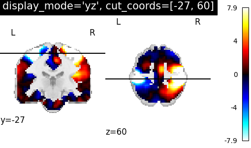
YZSlicer: Two views ‘coronal’ and ‘axial’ with coordinates
We can set display_mode='yz' to combine a coronal with an axial
view, which will return a YZSlicer
object.
plotting.plot_stat_map(
    stat_img,
    display_mode="yz",
    cut_coords=[-27, 60],
    title="display_mode='yz', cut_coords=[-27, 60]",
)
<nilearn.plotting.displays._slicers.YZSlicer object at 0x7f0c1c462d70>
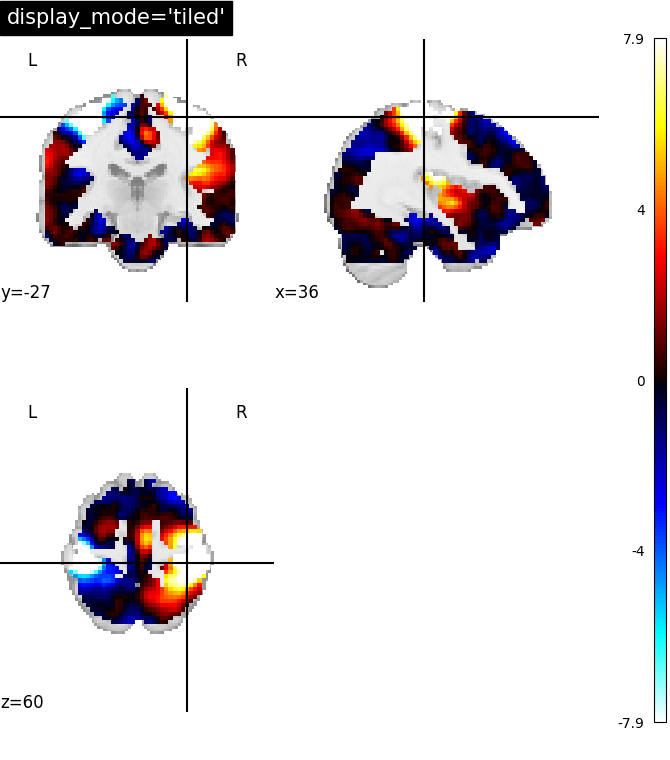
TiledSlicer: Three views in 2x2 fashion
If we want to combine three views in a 2x2 way, we can set
display_mode='tiled', which will combine sagittal, coronal, and axial
views. In this case, plot_stat_map will return
a TiledSlicer object.
plotting.plot_stat_map(
    stat_img,
    display_mode="tiled",
    cut_coords=[36, -27, 60],
    title="display_mode='tiled'",
)
<nilearn.plotting.displays._slicers.TiledSlicer object at 0x7f0c1885a980>
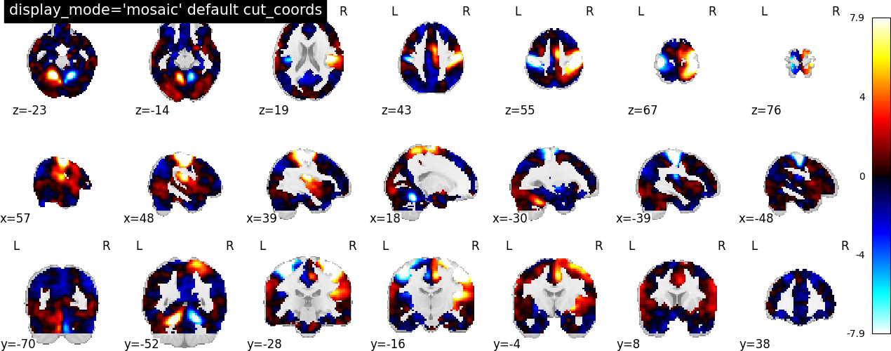
MosaicSlicer: Three views along multiple rows and columns
If we set display_mode='mosaic', we can easily combine sagittal,
coronal, and axial views with different rows and columns. In this
situation, plot_stat_map returns a
MosaicSlicer object.
Below we show the default option cut_coords=None.
plotting.plot_stat_map(
    stat_img,
    display_mode="mosaic",
    title="display_mode='mosaic' default cut_coords",
)
<nilearn.plotting.displays._slicers.MosaicSlicer object at 0x7f0c1ca28fd0>
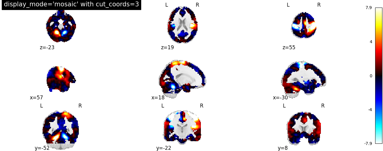
We can also set the number of slices to be the same across views.
In this case, we can specify it as an integer, i.e. cut_coords=3.
plotting.plot_stat_map(
    stat_img,
    display_mode="mosaic",
    cut_coords=3,
    title="display_mode='mosaic' with cut_coords=3",
)
<nilearn.plotting.displays._slicers.MosaicSlicer object at 0x7f0bf645cca0>
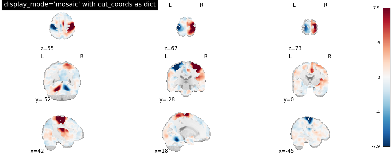
It can be the case that we want to display a different number of cuts in
each view. In this situation, we still set display_mode='mosaic', but
we specify the number of slices as a tuple of length 3.
plotting.plot_stat_map(
    stat_img,
    display_mode="mosaic",
    cut_coords=(5, 4, 10),
    title="display_mode='mosaic' with cut_coords as tuple",
)
<nilearn.plotting.displays._slicers.MosaicSlicer object at 0x7f0bf2f27b80>
It is also possible to specify cut positions in each direction.
In this situation, we still set display_mode='mosaic', but
we specify the cut positions of slices as a dictionary with keys
“x”, “y”, “z” and values as list of cut positions in that direction.
plotting.plot_stat_map(
    stat_img,
    display_mode="mosaic",
    cut_coords={"x": [42, 18, -45], "y": [-52, -28, 0], "z": [55, 67, 73]},
    title="display_mode='mosaic' with cut_coords as dict",
)
<nilearn.plotting.displays._slicers.MosaicSlicer object at 0x7f0c189f7df0>
Display object’s features
In this second part, we demonstrate how to interact with the obtained figures. More precisely, we will show how to use specific methods of the display objects which can be helpful in projecting brain imaging results for further interpretation.
# Import image processing tool for basic processing of functional brain image
from nilearn import image

# Compute voxel-wise mean functional image across time dimension. Now we have
# functional image in 3D assigned in mean_haxby_img
mean_haxby_img = image.mean_img(haxby_func_filename)
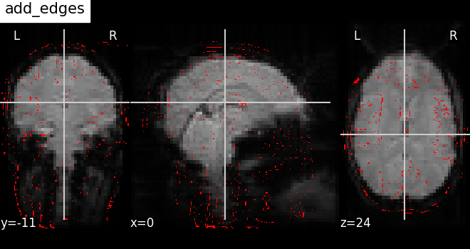
Overlay anatomical image as edges: add_edges
Now let us see how to use the method
add_edges for checking
coregistration by overlaying anatomical image as edges (red) on top of
mean functional image (background), both being of same subject.
First, we call the plot_anat plotting function,
with a background image as first argument, in this case the mean
fMRI image.
We then use the add_edges
method. The first argument is the anatomical image and, by default,
edges will be displayed in red (‘r’). To choose a different color, use
the color argument.
display = plotting.plot_anat(mean_haxby_img, title="add_edges")
display.add_edges(haxby_anat_filename, color="r")
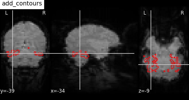
Plot the outline of a mask: add_contours
Here, we show how to plot the outline of a mask (in red) on top of the
mean EPI image with the method
add_contours.
This method is useful for region specific interpretation of brain images
As before, we call the plot_anat function with a
background image as first argument, in this case the mean fMRI
image, and argument cut_coords as a list for manual cuts with coordinates
pointing at masked brain regions.
We then use the add_contours
method of the display object returned by
plot_anat. We provide the path to a mask image
from the Haxby dataset as the first argument, and we provide levels as
a list of values to select particular levels in the contour to display.
We also specify colors='r' to display edges in red (See function
contour to use more options).
display = plotting.plot_anat(
    mean_haxby_img, title="add_contours", cut_coords=[-34, -39, -9]
)

display.add_contours(haxby_mask_filename, levels=[0.5], colors="r")
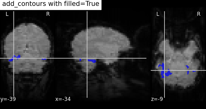
Here, we plot the outline of the mask (in blue) with color fillings using
the same method add_contours.
By default, no color fillings will be shown using
add_contours. To see
contours with color fillings, use argument filled=True. Here, contour
colors are changed to blue ‘b’, and we specify alpha=0.7 to set the
transparency of the fillings.
See function contourf to use more options (given
that filled should be True).
display = plotting.plot_anat(
    mean_haxby_img,
    title="add_contours with filled=True",
    cut_coords=[-34, -39, -9],
)

display.add_contours(
    haxby_mask_filename, filled=True, alpha=0.7, levels=[0.5], colors="b"
)
/home/runner/work/nilearn/nilearn/examples/01_plotting/plot_demo_more_plotting.py:345: UserWarning:

kwargs['alpha']=0.7 detected in parameters.
Overriding with transparency=None.
To suppress this warning pass your 'alpha' value via the 'transparency' parameter.
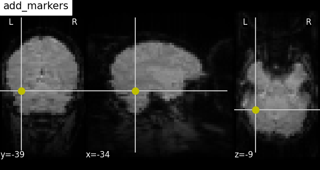
Plotting seeds: add_markers
Plotting seed regions of interest as spheres using method
add_markers
with MNI coordinates of interest.
The coordinates of the seed regions should be specified as the first
argument, and second argument marker_color is used to denote the
color of the sphere (in this case yellow ‘y’). The third argument
marker_size is used to control the size of the sphere.
display = plotting.plot_anat(
    mean_haxby_img, title="add_markers", cut_coords=[-34, -39, -9]
)
coords = [(-34, -39, -9)]
display.add_markers(coords, marker_color="y", marker_size=100)
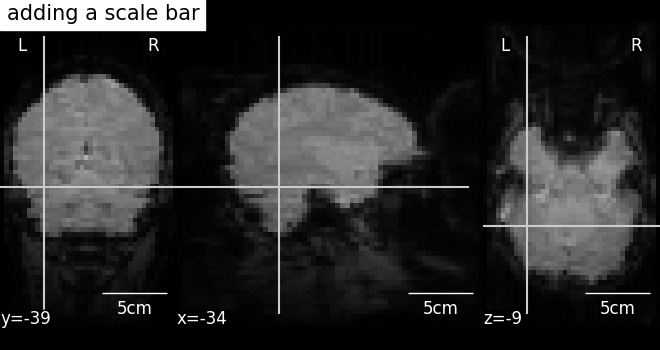
Annotate plots: annotate
It is possible to alter the default annotations of plots, using the
method annotate of the
display objects. For example, we can add a scale bar at the bottom
right of each view:
display = plotting.plot_anat(
    mean_haxby_img, title="adding a scale bar", cut_coords=[-34, -39, -9]
)
display.annotate(scalebar=True)
Further configuration can be achieved by setting scale_* keyword args.
For instance, we can change the units to mm, or use a different
scale bar size.
display = plotting.plot_anat(
    mean_haxby_img, title="adding a scale bar", cut_coords=[-34, -39, -9]
)
display.annotate(scalebar=True, scale_size=25, scale_units="mm")

Save plots to a file: savefig
Finally, we can save a plot to file in two different ways:
First, we can save the contrast maps plotted with the function
plot_stat_map using the built-in parameter
output_file. We provide the filename and the file extension as
a string (supported extensions are .png, .pdf, .svg).
from pathlib import Path

output_dir = Path.cwd() / "results" / "plot_demo_more_plotting"
output_dir.mkdir(exist_ok=True, parents=True)
print(f"Output will be saved to: {output_dir}")

plotting.plot_stat_map(
    stat_img,
    title="Using plot_stat_map output_file",
    output_file=output_dir / "plot_stat_map.png",
)
Output will be saved to: /home/runner/work/nilearn/nilearn/examples/01_plotting/results/plot_demo_more_plotting
A second way to save plots is by using the method
savefig of the display
object returned.
display = plotting.plot_stat_map(stat_img, title="Using display savefig")

display.savefig(output_dir / "plot_stat_map_from_display.png")

# In non-interactive settings make sure you close your displays
display.close()

plotting.show()
Total running time of the script: (0 minutes 16.667 seconds)
Estimated memory usage: 1053 MB