Loading and plotting of a cortical surface atlas

The Destrieux parcellation (Destrieux et al.[1]) in fsaverage5 space as distributed with Freesurfer is used as the chosen atlas.

The plot_surf_roi function is used to plot the parcellation on the pial surface.

See Plotting brain images for more details.

Data fetcher

Retrieve destrieux parcellation in fsaverage5 space from nilearn and create a SurfaceImage instance with it.

from nilearn.datasets import (
    fetch_atlas_surf_destrieux,
    load_fsaverage,
    load_fsaverage_data,
)
from nilearn.surface import SurfaceImage

fsaverage = load_fsaverage("fsaverage5")
destrieux = fetch_atlas_surf_destrieux()
destrieux_atlas = SurfaceImage(
    mesh=fsaverage["pial"],
    data={
        "left": destrieux["map_left"],
        "right": destrieux["map_right"],
    },
)

# The labels are stored as bytes for the Destrieux atlas.
# For convenience we decode them to string.
labels = [x.decode("utf-8") for x in destrieux.labels]

# Retrieve fsaverage5 surface dataset for the plotting background.
# It contains the surface template as pial and inflated version.
fsaverage_meshes = load_fsaverage()

# The fsaverage meshes contains the FileMesh objects:
print(f"{fsaverage_meshes['pial'].parts['left']=}")
print(f"{fsaverage_meshes['inflated'].parts['left']=}")

# The fsaverage data contains file names pointing to the file locations
# The sulcal depth maps will be is used for shading.
fsaverage_sulcal = load_fsaverage_data(data_type="sulcal")
print(f"{fsaverage_sulcal=}")

[get_dataset_dir] Dataset found in /home/remi/nilearn_data/destrieux_surface
fsaverage_meshes['pial'].parts['left']=<FileMesh with 10242 vertices and 20480 faces.>
fsaverage_meshes['inflated'].parts['left']=<FileMesh with 10242 vertices and 20480 faces.>
fsaverage_sulcal=<SurfaceImage (20484,)>

Visualization

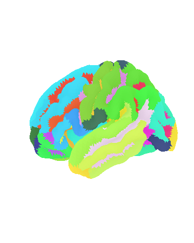
Destrieux parcellation on pial surface

from nilearn.plotting import plot_surf_roi, show

plot_surf_roi(
    roi_map=destrieux_atlas,
    hemi="left",
    view="lateral",
    bg_map=fsaverage_sulcal,
    bg_on_data=True,
    darkness=0.5,
    title="Destrieux parcellation on sulcal surface",
)

<Figure size 400x500 with 1 Axes>

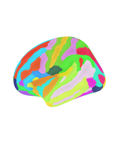
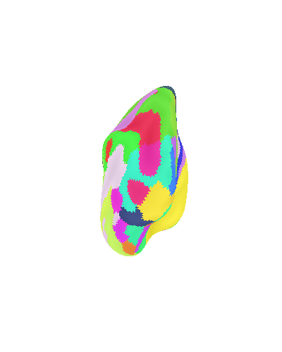
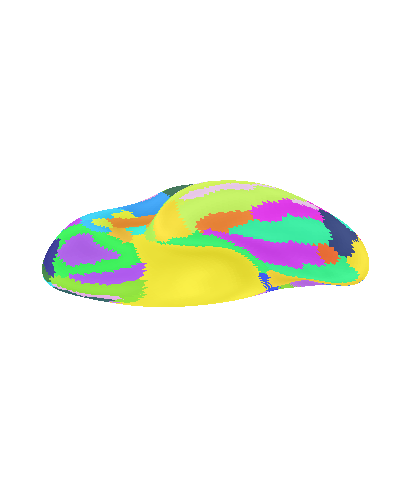
Destrieux parcellation on inflated surface with different views

for view in ["lateral", "posterior", "ventral"]:
    plot_surf_roi(
        surf_mesh=fsaverage_meshes["inflated"],
        roi_map=destrieux_atlas,
        hemi="left",
        view=view,
        bg_map=fsaverage_sulcal,
        bg_on_data=True,
        darkness=0.5,
        title=f"Destrieux parcellation on inflated surface\n{view} view",
    )

show()

• 
• 
• 

Destrieux parcellation with custom view: explicitly set angle

elev, azim = 210.0, 90.0  # appropriate for visualizing, e.g., the OTS
plot_surf_roi(
    surf_mesh=fsaverage_meshes["inflated"],
    roi_map=destrieux_atlas,
    hemi="left",
    view=(elev, azim),
    bg_map=fsaverage_sulcal,
    bg_on_data=True,
    darkness=0.5,
    title="Arbitrary view of Destrieux parcellation",
)

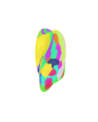
<Figure size 400x500 with 1 Axes>

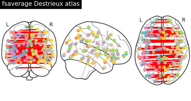
Display connectome from surface parcellation

The following code extracts 3D coordinates of surface parcels (also known as labels in the Freesurfer naming convention). To do so we get the pial surface of fsaverage subject, get the vertices contained in each parcel and compute the mean location to obtain the coordinates.

import numpy as np

from nilearn.plotting import plot_connectome, view_connectome

coordinates = []
for hemi in ["left", "right"]:
    data = destrieux_atlas.data.parts[hemi]
    mesh_coordinates = destrieux_atlas.mesh.parts[hemi].coordinates
    coordinates.extend(
        np.mean(mesh_coordinates[data == k], axis=0)
        for k, label in enumerate(labels)
        if "Unknown" not in str(label)
    )
# 3D coordinates of parcels
coordinates = np.array(coordinates)

# We now make a synthetic connectivity matrix that connects labels
# between left and right hemispheres.
n_parcels = len(coordinates)
corr = np.zeros((n_parcels, n_parcels))
n_parcels_hemi = n_parcels // 2
corr[np.arange(n_parcels_hemi), np.arange(n_parcels_hemi) + n_parcels_hemi] = 1
corr = corr + corr.T

plot_connectome(
    adjacency_matrix=corr,
    node_coords=coordinates,
    edge_threshold="90%",
    title="Connectome Destrieux atlas",
)
show()

3D visualization in a web browser

An alternative to plot_surf_roi is to use view_surf for more interactive visualizations in a web browser. See 3D Plots of statistical maps or atlases on the cortical surface for more details.

from nilearn.plotting import view_surf

view = view_surf(
    surf_mesh=fsaverage_meshes["inflated"],
    surf_map=destrieux_atlas,
    cmap="gist_ncar",
    symmetric_cmap=False,
    colorbar=False,
)
# In a Jupyter notebook, if ``view`` is the output of a cell,
# it will be displayed below the cell
view

# uncomment this to open the plot in a web browser:
# view.open_in_browser()

you can also use view_connectome to open an interactive view of the connectome.

view = view_connectome(
    corr,
    coordinates,
    edge_threshold="90%",
    colorbar=False,
)

# uncomment this to open the plot in a web browser:
# view.open_in_browser()
view

References

[1]

Christophe Destrieux, Bruce Fischl, Anders Dale, and Eric Halgren. Automatic parcellation of human cortical gyri and sulci using standard anatomical nomenclature. NeuroImage, 53(1):1–15, 2010. URL: https://www.sciencedirect.com/science/article/pii/S1053811910008542, doi:https://doi.org/10.1016/j.neuroimage.2010.06.010.

Estimated memory usage: 219 MB