Extract signals on spheres and plot a connectome

This example shows how to extract signals from spherical regions. We show how to build spheres around user-defined coordinates, as well as centered on coordinates from the Power-264 atlas (Power et al.[1]), and the Dosenbach-160 atlas (Dosenbach et al.[2]).

We estimate connectomes using two different methods: sparse inverse covariance and partial_correlation, to recover the functional brain networks structure.

We’ll start by extracting signals from Default Mode Network regions and computing a connectome from them.

Note

If you are using Nilearn with a version older than 0.9.0, then you should either upgrade your version or import maskers from the input_data module instead of the maskers module.

That is, you should manually replace in the following example all occurrences of:

from nilearn.maskers import NiftiMasker

with:

from nilearn.input_data import NiftiMasker

from nilearn import datasets, plotting

Retrieve the brain development fMRI dataset

We are going to use a subject from the development functional connectivity dataset.

dataset = datasets.fetch_development_fmri(n_subjects=10)

# print basic information on the dataset
print(f"First subject functional nifti image (4D) is at: {dataset.func[0]}")

[get_dataset_dir] Dataset found in /home/remi/nilearn_data/development_fmri
[get_dataset_dir] Dataset found in /home/remi/nilearn_data/development_fmri/development_fmri
[get_dataset_dir] Dataset found in /home/remi/nilearn_data/development_fmri/development_fmri
First subject functional nifti image (4D) is at: /home/remi/nilearn_data/development_fmri/development_fmri/sub-pixar123_task-pixar_space-MNI152NLin2009cAsym_desc-preproc_bold.nii.gz

Coordinates of Default Mode Network

dmn_coords = [(0, -52, 18), (-46, -68, 32), (46, -68, 32), (1, 50, -5)]
labels = [
    "Posterior Cingulate Cortex",
    "Left Temporoparietal junction",
    "Right Temporoparietal junction",
    "Medial prefrontal cortex",
]

Extracts signal from sphere around DMN seeds

We can compute the mean signal within spheres of a fixed radius around a sequence of (x, y, z) coordinates with the object nilearn.maskers.NiftiSpheresMasker. The resulting signal is then prepared by the masker object: Detrended, band-pass filtered and standardized to 1 variance.

from nilearn.maskers import NiftiSpheresMasker

masker = NiftiSpheresMasker(
    dmn_coords,
    radius=8,
    detrend=True,
    standardize="zscore_sample",
    standardize_confounds="zscore_sample",
    low_pass=0.1,
    high_pass=0.01,
    t_r=2,
    memory="nilearn_cache",
    memory_level=1,
    verbose=2,
    clean__butterworth__padtype="even",  # kwarg to modify Butterworth filter
)

# Additionally, we pass confound information to ensure our extracted
# signal is cleaned from confounds.

func_filename = dataset.func[0]
confounds_filename = dataset.confounds[0]

time_series = masker.fit_transform(
    func_filename, confounds=[confounds_filename]
)

________________________________________________________________________________
[Memory] Calling nilearn.maskers.base_masker._filter_and_extract...
_filter_and_extract('/home/remi/nilearn_data/development_fmri/development_fmri/sub-pixar123_task-pixar_space-MNI152NLin2009cAsym_desc-preproc_bold.nii.gz',
<nilearn.maskers.nifti_spheres_masker._ExtractionFunctor object at 0x740cdfd7a3d0>,
{ 'allow_overlap': False,
  'clean_kwargs': {'butterworth__padtype': 'even'},
  'detrend': True,
  'dtype': None,
  'high_pass': 0.01,
  'high_variance_confounds': False,
  'low_pass': 0.1,
  'mask_img': None,
  'radius': 8,
  'reports': True,
  'seeds': [(0, -52, 18), (-46, -68, 32), (46, -68, 32), (1, 50, -5)],
  'smoothing_fwhm': None,
  'standardize': 'zscore_sample',
  'standardize_confounds': 'zscore_sample',
  't_r': 2}, confounds=[ '/home/remi/nilearn_data/development_fmri/development_fmri/sub-pixar123_task-pixar_desc-reducedConfounds_regressors.tsv'], sample_mask=None, dtype=None, memory=Memory(location=nilearn_cache/joblib), memory_level=1, verbose=2)
[NiftiSpheresMasker.wrapped] Loading data from
/home/remi/nilearn_data/development_fmri/development_fmri/sub-pixar123_task-pixar_space-MNI152NLin2009cAsym_desc-preproc_bold.nii.gz
[NiftiSpheresMasker.wrapped] Extracting region signals
[NiftiSpheresMasker.wrapped] Cleaning extracted signals
_______________________________________________filter_and_extract - 1.9s, 0.0min

Display spheres summary report

By default all spheres are displayed. This can be tweaked by passing an integer or list/array of indices to the displayed_spheres argument of generate_report.

report = masker.generate_report()
report

NiftiSpheresMasker Class for masking of Niimg-like objects using seeds. NiftiSpheresMasker is useful when data from given seeds should be extracted. Use case: summarize brain signals from seeds that were obtained from prior knowledge.

Previous Sphere

All Spheres

Sphere

Next Sphere

This reports shows the regions defined by the spheres of the masker.

The masker has 4 spheres in total (displayed together on the first image).

They can be individually browsed using Previous and Next buttons.

Regions summary

seed number	coordinates	position	radius	size (in mm^3)	size (in voxels)	relative size (in %)
0	[0, -52, 18]	[24 20 24]	8	2144.66	not implemented	not implemented
1	[-46, -68, 32]	[12 16 28]	8	2144.66	not implemented	not implemented
2	[46, -68, 32]	[36 16 28]	8	2144.66	not implemented	not implemented
3	[1, 50, -5]	[24 46 18]	8	2144.66	not implemented	not implemented

Parameters

Parameter	Value
allow_overlap	False
detrend	True
dtype	None
high_pass	0.01
high_variance_confounds	False
low_pass	0.1
mask_img	None
memory	Memory(location=nilearn_cache/joblib)
memory_level	1
radius	8
reports	True
seeds	[(0, -52, 18), (-46, -68, 32), (46, -68, 32), (1, 50, -5)]
smoothing_fwhm	None
standardize	zscore_sample
standardize_confounds	zscore_sample
t_r	2
verbose	2

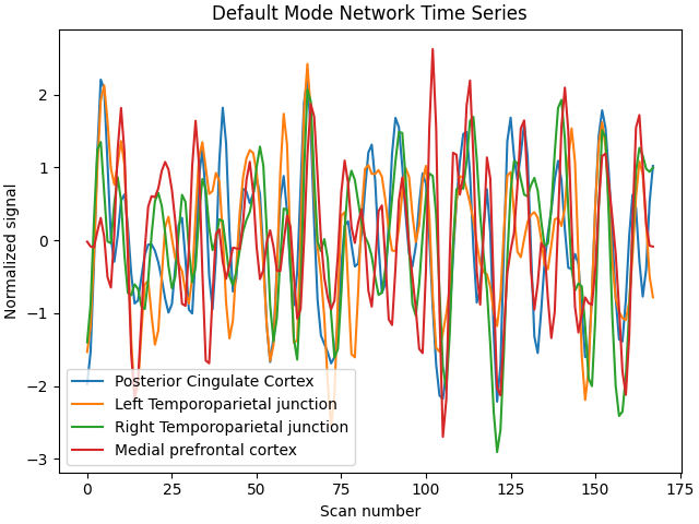
Display time series

import matplotlib.pyplot as plt

plt.figure(constrained_layout=True)

for time_serie, label in zip(time_series.T, labels):
    plt.plot(time_serie, label=label)

plt.title("Default Mode Network Time Series")
plt.xlabel("Scan number")
plt.ylabel("Normalized signal")
plt.legend()

<matplotlib.legend.Legend object at 0x740d1ace89a0>

Compute partial correlation matrix

Using object nilearn.connectome.ConnectivityMeasure: its default covariance estimator is Ledoit-Wolf, allowing to obtain accurate partial correlations.

from nilearn.connectome import ConnectivityMeasure

connectivity_measure = ConnectivityMeasure(
    kind="partial correlation",
    standardize="zscore_sample",
)
partial_correlation_matrix = connectivity_measure.fit_transform([time_series])[
    0
]

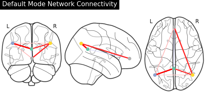
Display connectome

We display the graph of connections with :func: nilearn.plotting.plot_connectome.

plotting.plot_connectome(
    partial_correlation_matrix,
    dmn_coords,
    title="Default Mode Network Connectivity",
)

<nilearn.plotting.displays._projectors.OrthoProjector object at 0x740d1d73ec70>

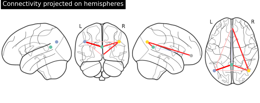
Display connectome with hemispheric projections. Notice (0, -52, 18) is included in both hemispheres since x == 0.

plotting.plot_connectome(
    partial_correlation_matrix,
    dmn_coords,
    title="Connectivity projected on hemispheres",
    display_mode="lyrz",
)

plotting.show()

3D visualization in a web browser

An alternative to nilearn.plotting.plot_connectome is to use nilearn.plotting.view_connectome, which gives more interactive visualizations in a web browser. See 3D Plots of connectomes for more details.

view = plotting.view_connectome(partial_correlation_matrix, dmn_coords)

# In a Jupyter notebook, if ``view`` is the output of a cell, it will
# be displayed below the cell
view

# uncomment this to open the plot in a web browser:
# view.open_in_browser()

Extract signals on spheres from an atlas

Next, instead of supplying our own coordinates, we will use coordinates generated at the center of mass of regions from two different atlases. This time, we’ll use a different correlation measure.

First we fetch the coordinates of the Power atlas

power = datasets.fetch_coords_power_2011(legacy_format=False)
print(f"Power atlas comes with {power.keys()}.")

Power atlas comes with dict_keys(['rois', 'description']).

Note

You can retrieve the coordinates for any atlas, including atlases not included in nilearn, using nilearn.plotting.find_parcellation_cut_coords.

Compute within spheres averaged time-series

We collect the regions coordinates in a numpy array

import numpy as np

coords = np.vstack((power.rois["x"], power.rois["y"], power.rois["z"])).T

print(f"Stacked power coordinates in array of shape {coords.shape}.")

Stacked power coordinates in array of shape (264, 3).

and define spheres masker, with small enough radius to avoid regions overlap.

spheres_masker = NiftiSpheresMasker(
    seeds=coords,
    smoothing_fwhm=6,
    radius=5.0,
    detrend=True,
    standardize="zscore_sample",
    standardize_confounds="zscore_sample",
    low_pass=0.1,
    high_pass=0.01,
    t_r=2,
)

timeseries = spheres_masker.fit_transform(
    func_filename, confounds=confounds_filename
)

Estimate correlations

We start by estimating the signal covariance matrix. Here the number of ROIs exceeds the number of samples,

print(f"time series has {timeseries.shape[0]} samples")

time series has 168 samples

in which situation the graphical lasso sparse inverse covariance estimator captures well the covariance structure.

from sklearn.covariance import GraphicalLassoCV

covariance_estimator = GraphicalLassoCV(cv=3, verbose=1)

We just fit our regions signals into the GraphicalLassoCV object

covariance_estimator.fit(timeseries)

[Parallel(n_jobs=1)]: Using backend SequentialBackend with 1 concurrent workers.
[Parallel(n_jobs=1)]: Done   3 out of   3 | elapsed:   12.5s finished
[GraphicalLassoCV] Done refinement  1 out of 4:  12s
[Parallel(n_jobs=1)]: Using backend SequentialBackend with 1 concurrent workers.
[Parallel(n_jobs=1)]: Done   3 out of   3 | elapsed:   46.8s finished
[GraphicalLassoCV] Done refinement  2 out of 4:  59s
[Parallel(n_jobs=1)]: Using backend SequentialBackend with 1 concurrent workers.
[Parallel(n_jobs=1)]: Done   3 out of   3 | elapsed:  1.0min finished
[GraphicalLassoCV] Done refinement  3 out of 4:  120s
[Parallel(n_jobs=1)]: Using backend SequentialBackend with 1 concurrent workers.
[Parallel(n_jobs=1)]: Done   3 out of   3 | elapsed:  1.0min finished
[GraphicalLassoCV] Done refinement  4 out of 4:  182s
/home/remi/github/nilearn/nilearn_doc_build/.tox/doc/lib/python3.9/site-packages/numpy/core/_methods.py:232: RuntimeWarning:

invalid value encountered in subtract

GraphicalLassoCV(cv=3, verbose=1)

In a Jupyter environment, please rerun this cell to show the HTML representation or trust the notebook.
On GitHub, the HTML representation is unable to render, please try loading this page with nbviewer.org.

and get the ROI-to-ROI covariance matrix.

matrix = covariance_estimator.covariance_
print(f"Covariance matrix has shape {matrix.shape}.")

Covariance matrix has shape (264, 264).

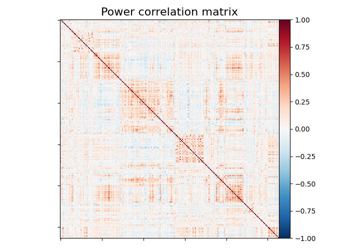
Plot matrix, graph, and strength

We use :func: nilearn.plotting.plot_matrix to visualize our correlation matrix and display the graph of connections with nilearn.plotting.plot_connectome.

plotting.plot_matrix(
    matrix,
    vmin=-1.0,
    vmax=1.0,
    colorbar=True,
    title="Power correlation matrix",
)

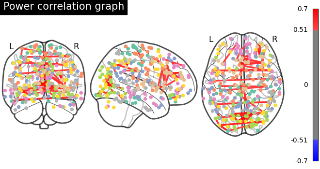
# Tweak edge_threshold to keep only the strongest connections.
plotting.plot_connectome(
    matrix,
    coords,
    title="Power correlation graph",
    edge_threshold="99.8%",
    node_size=20,
    colorbar=True,
)

• 
• 

<nilearn.plotting.displays._projectors.OrthoProjector object at 0x740d1d6dd700>

Note

Note the 1. on the matrix diagonal: These are the signals variances, set to 1. by the spheres_masker. Hence the covariance of the signal is a correlation matrix.

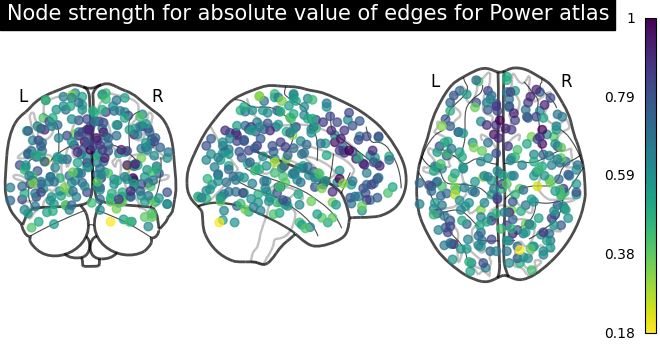
Sometimes, the information in the correlation matrix is overwhelming and aggregating edge strength from the graph would help. Use the function nilearn.plotting.plot_markers to visualize this information.

# calculate normalized, absolute strength for each node
node_strength = np.sum(np.abs(matrix), axis=0)
node_strength /= np.max(node_strength)

plotting.plot_markers(
    node_strength,
    coords,
    title="Node strength for absolute value of edges for Power atlas",
)

<nilearn.plotting.displays._projectors.OrthoProjector object at 0x740cf17c52b0>

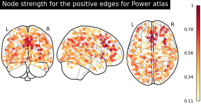
From the correlation matrix, we observe that there is a positive and negative structure. We could make two different plots, one for the positive and one for the negative structure.

from matplotlib.pyplot import cm

# clip connectivity matrix to preserve positive and negative edges
positive_edges = np.clip(matrix, 0, matrix.max())
negative_edges = np.clip(matrix, matrix.min(), 0)

# calculate strength for positive edges
node_strength_positive = np.sum(np.abs(positive_edges), axis=0)
node_strength_positive /= np.max(node_strength_positive)

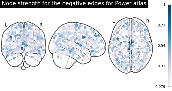
# calculate strength for negative edges
node_strength_negative = np.sum(np.abs(negative_edges), axis=0)
node_strength_negative /= np.max(node_strength_negative)

# plot nodes' strength for positive edges
plotting.plot_markers(
    node_strength_positive,
    coords,
    title="Node strength for the positive edges for Power atlas",
    node_cmap=cm.YlOrRd,
)

# plot nodes' strength for negative edges
plotting.plot_markers(
    node_strength_negative,
    coords,
    title="Node strength for the negative edges for Power atlas",
    node_cmap=cm.PuBu,
)

• 
• 

<nilearn.plotting.displays._projectors.OrthoProjector object at 0x740d1d1dca00>

Connectome extracted from Dosenbach’s atlas

We repeat the same steps for Dosenbach’s atlas.

dosenbach = datasets.fetch_coords_dosenbach_2010(legacy_format=False)

coords = np.vstack(
    (
        dosenbach.rois["x"],
        dosenbach.rois["y"],
        dosenbach.rois["z"],
    )
).T

spheres_masker = NiftiSpheresMasker(
    seeds=coords,
    smoothing_fwhm=6,
    radius=4.5,
    detrend=True,
    standardize="zscore_sample",
    standardize_confounds="zscore_sample",
    low_pass=0.1,
    high_pass=0.01,
    t_r=2,
)

timeseries = spheres_masker.fit_transform(
    func_filename, confounds=confounds_filename
)

covariance_estimator = GraphicalLassoCV()
covariance_estimator.fit(timeseries)
matrix = covariance_estimator.covariance_

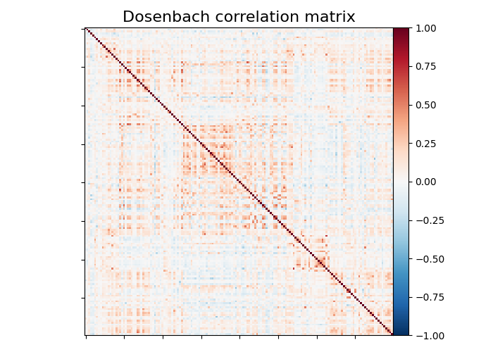
plotting.plot_matrix(
    matrix,
    vmin=-1.0,
    vmax=1.0,
    colorbar=True,
    title="Dosenbach correlation matrix",
)

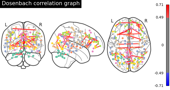
plotting.plot_connectome(
    matrix,
    coords,
    title="Dosenbach correlation graph",
    edge_threshold="99.7%",
    node_size=20,
    colorbar=True,
)


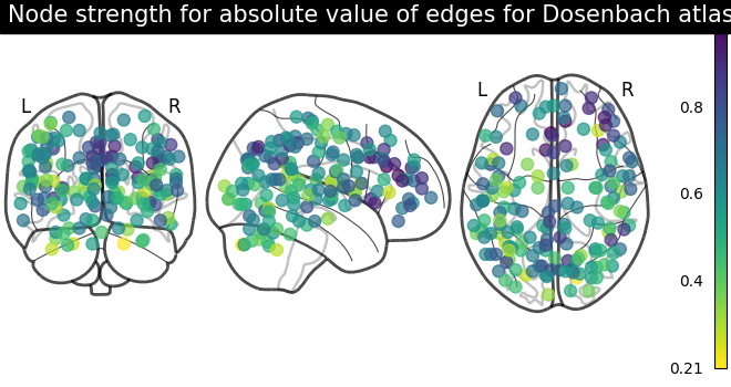
# calculate average strength for each node
node_strength = np.sum(np.abs(matrix), axis=0)
node_strength /= np.max(node_strength)

plotting.plot_markers(
    node_strength,
    coords,
    title="Node strength for absolute value of edges for Dosenbach atlas",
)

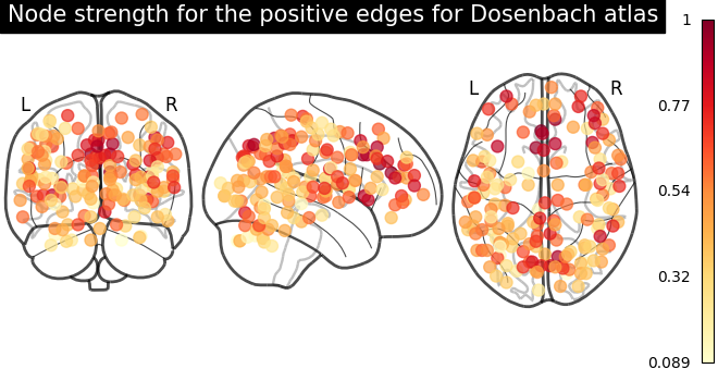
# clip connectivity matrix to preserve positive and negative edges
positive_edges = np.clip(matrix, 0, matrix.max())
negative_edges = np.clip(matrix, matrix.min(), 0)

# calculate strength for positive and edges
node_strength_positive = np.sum(np.abs(positive_edges), axis=0)
node_strength_positive /= np.max(node_strength_positive)
node_strength_negative = np.sum(np.abs(negative_edges), axis=0)
node_strength_negative /= np.max(node_strength_negative)

# plot nodes' strength for positive edges
plotting.plot_markers(
    node_strength_positive,
    coords,
    title="Node strength for the positive edges for Dosenbach atlas",
    node_cmap=cm.YlOrRd,
)

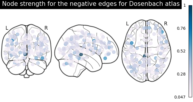
# plot nodes' strength for negative edges
plotting.plot_markers(
    node_strength_negative,
    coords,
    title="Node strength for the negative edges for Dosenbach atlas",
    node_cmap=cm.PuBu,
)

• 
• 
• 
• 
• 

/home/remi/github/nilearn/nilearn_doc_build/.tox/doc/lib/python3.9/site-packages/numpy/core/_methods.py:232: RuntimeWarning:

invalid value encountered in subtract


<nilearn.plotting.displays._projectors.OrthoProjector object at 0x740d1a611730>

We can easily identify the Dosenbach’s networks from the matrix blocks.

print(f"Dosenbach networks names are {np.unique(dosenbach.networks)}")

plotting.show()

Dosenbach networks names are ['cerebellum' 'cingulo-opercular' 'default' 'fronto-parietal' 'occipital'
 'sensorimotor']

References

[1]

Jonathan D. Power, Alexander L. Cohen, Steven M. Nelson, Gagan S. Wig, Kelly Anne Barnes, Jessica A. Church, Alecia C. Vogel, Timothy O. Laumann, Fran M. Miezin, Bradley L. Schlaggar, and Steven E. Petersen. Functional network organization of the human brain. Neuron, 72(4):665–678, Nov 2011. URL: https://doi.org/10.1016/j.neuron.2011.09.006, doi:10.1016/j.neuron.2011.09.006.

[2]

Nico U. F. Dosenbach, Binyam Nardos, Alexander L. Cohen, Damien A. Fair, Jonathan D. Power, Jessica A. Church, Steven M. Nelson, Gagan S. Wig, Alecia C. Vogel, Christina N. Lessov-Schlaggar, Kelly Anne Barnes, Joseph W. Dubis, Eric Feczko, Rebecca S. Coalson, John R. Pruett, Deanna M. Barch, Steven E. Petersen, and Bradley L. Schlaggar. Prediction of individual brain maturity using fmri. Science, 329(5997):1358–1361, 2010. URL: https://science.sciencemag.org/content/329/5997/1358, arXiv:https://science.sciencemag.org/content/329/5997/1358.full.pdf, doi:10.1126/science.1194144.

See also

• Comparing connectomes on different reference atlases

• Group Sparse inverse covariance for multi-subject connectome # noqa: E501

Estimated memory usage: 1092 MB